ssd原理及代码实现详解

• 2019 年 10 月 29 日
• 笔记

通过https://github.com/amdegroot/ssd.pytorch,结合论文https://arxiv.org/abs/1512.02325来理解ssd.

ssd由三部分组成:

• base
• extra
• predict
  base原论文里用的是vgg16去掉全连接层.
  
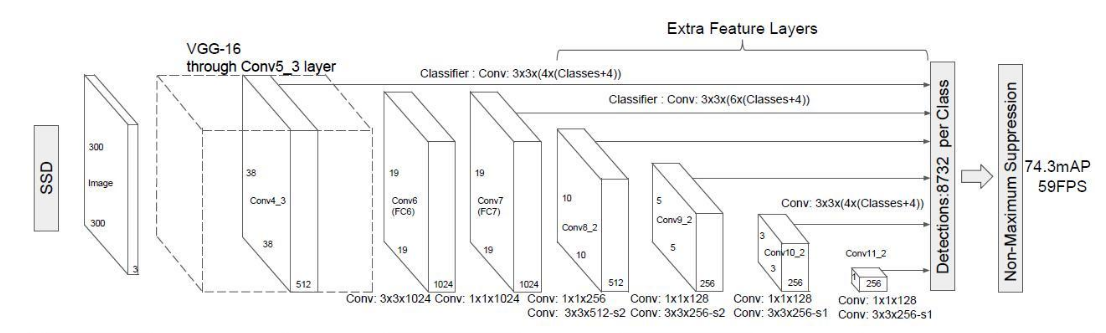
  base + extra完成特征提取的功能.得到不同size的feature map,基于这些feature maps,我们再用不同的卷积核去卷积,分别完成类别预测和坐标预测.

基础特征提取网络

特征提取网络由两部分组成

• vgg16
• extra layer

vgg16变种

vgg16结构:

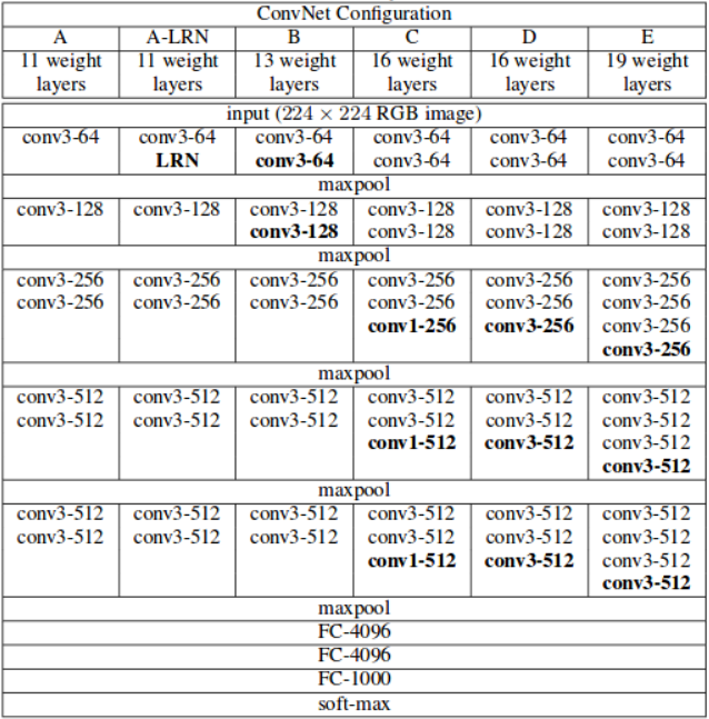
将vgg16的全连接层用卷积层换掉.

代码实现

ssd.py中

base = {      '300': [64, 64, 'M', 128, 128, 'M', 256, 256, 256, 'C', 512, 512, 512, 'M',              512, 512, 512],      '512': [],  }  extras = {      '300': [256, 'S', 512, 128, 'S', 256, 128, 256, 128, 256],      '512': [],  }  }

定义了每一层的卷积核的数量.其中’M’,’C’均代表maxpool池化层.只是’C’会使用 ceil instead of floor to compute the output shape.
参见https://pytorch.org/docs/stable/nn.html#maxpool2d

def vgg(cfg, i, batch_norm=False):      layers = []      in_channels = i      for v in cfg:          if v == 'M':              layers += [nn.MaxPool2d(kernel_size=2, stride=2)]          elif v == 'C':              layers += [nn.MaxPool2d(kernel_size=2, stride=2, ceil_mode=True)]          else:              conv2d = nn.Conv2d(in_channels, v, kernel_size=3, padding=1)              if batch_norm:                  layers += [conv2d, nn.BatchNorm2d(v), nn.ReLU(inplace=True)]              else:                  layers += [conv2d, nn.ReLU(inplace=True)]              in_channels = v      pool5 = nn.MaxPool2d(kernel_size=3, stride=1, padding=1)      conv6 = nn.Conv2d(512, 1024, kernel_size=3, padding=6, dilation=6)      conv7 = nn.Conv2d(1024, 1024, kernel_size=1)      layers += [pool5, conv6,                 nn.ReLU(inplace=True), conv7, nn.ReLU(inplace=True)]      return layers  

这样就形成了一个基础的特征提取网络.前面的部分和vgg16一样的,全连接层换成了conv6+relu+conv7+relu.

extra layer

在前面得到的输出的基础上,继续做卷积,以得到更多不同尺寸的feature map.

代码实现

extras = {      '300': [256, 'S', 512, 128, 'S', 256, 128, 256, 128, 256],      '512': [],  }    def add_extras(cfg, i, batch_norm=False):      # Extra layers added to VGG for feature scaling      layers = []      in_channels = i      flag = False      for k, v in enumerate(cfg):          if in_channels != 'S':              if v == 'S':                  layers += [nn.Conv2d(in_channels, cfg[k + 1],                             kernel_size=(1, 3)[flag], stride=2, padding=1)]              else:                  layers += [nn.Conv2d(in_channels, v, kernel_size=(1, 3)[flag])]              flag = not flag          in_channels = v      return layers    add_extras(extras[str(size)], 1024)

[256, ‘S’, 512, 128, ‘S’, 256, 128, 256, 128, 256]用以创建layer.
如果是’S’的话,代表用的卷积核为3 x 3,否则为1 x 1,卷积核的数量为’S’下一个的数字.

这样的话,我们就构建出了extra layers.

多尺度检测multibox

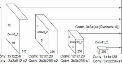
我们已经得到了很多layer的输出(称其为feature map).size有大有小. 那么现在我们就对某些层(conv4_3,conv7,conv8_2,conv9_2,conv10_2,conv11_2)的feature map再做卷积,得到类别和位置信息.
分别用2组3 x 3的卷积核去做卷积,一个负责预测类别,一个负责预测位置.卷积核的个数分别为boxnum x clasess_num,boxnum x 4(坐标由4个参数,中心坐标,box宽高即可确定).

即在m x m的feature map上做卷积我们会得到一个m x m x (boxnum x clasess_num) 和一个m x m x (boxnum x 4)的tensor.分别用以计算概率和框的位置.

代码实现

def multibox(vgg, extra_layers, cfg, num_classes):      loc_layers = []      conf_layers = []      vgg_source = [21, -2]      for k, v in enumerate(vgg_source):          loc_layers += [nn.Conv2d(vgg[v].out_channels,                                   cfg[k] * 4, kernel_size=3, padding=1)]          conf_layers += [nn.Conv2d(vgg[v].out_channels,                          cfg[k] * num_classes, kernel_size=3, padding=1)]      for k, v in enumerate(extra_layers[1::2], 2):          loc_layers += [nn.Conv2d(v.out_channels, cfg[k]                                   * 4, kernel_size=3, padding=1)]          conf_layers += [nn.Conv2d(v.out_channels, cfg[k]                                    * num_classes, kernel_size=3, padding=1)]      return vgg, extra_layers, (loc_layers, conf_layers)

其中每一个feature map预测几个box由下面变量给出.

mbox = {      '300': [4, 6, 6, 6, 4, 4],  # number of boxes per feature map location      '512': [],  }

在哪些layer的feature map上做预测,根据论文里是固定的,参见开头的ssd结构图.反映到代码里则为

vgg_source = [21, -2]  extra_layers[1::2]

即
中的conv4_3,conv7,conv8_2,conv9_2,conv10_2,conv11_2这六个layer的feature map.

先验框生成

你可以称之为priorbox/default box/anchor box都是一个意思.
我们先来讲先验框的原理.这个其实类似yolov3中的anchor box,我们基于这些shape的box去做预测.

priorbox和不同的feature map上做预测都是为了解决对不同尺寸的物体的检测问题.不同的feature map负责不同尺寸的目标.同时每一个feature map cell又负责该尺寸的不同宽高比的目标.

首先,不同的feature_map负责不同的尺寸.
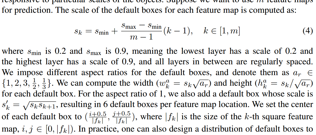
[s_k = s_{min} + frac{s_{max} – s_{min}}{m-1}(k-1), kin [1,m]]
对smin=0.2,smax=0.9.m=6(我们在6个layer的feature map上做检测), 因此就有 s={0.2,0.34,0.48,0.62,0.76,0.9}.
假设宽高比分别为(a_r ={1,2,3,1/2,1/3}),则对第二个feature map(19 x 19的这个,conv7),那么[w_k^a = s_ksqrt{a_r},h_k^a = s_k/sqrt{a_r}],我们计算宽高比为1的box,则得到的box为(0.2,0.2).模型的输入图像尺寸是(300,300),那么相应的box为(60,60).依次类推,可以得到其余的deafult box的shape共6个.(对宽高比为1的box,额外多计算一个(s_k^prime)的box出来). 从而我们得到了这一个feature map负责预测的不同形状的box

如图:

那么对于conv4_3这个layer而言的话,我们设定的deafault box数量是4,于是我们最终就有38 x 38 x 4个box.我们在这些box的基础上去预测我们的box.

我们对不同层的default box的数量设定是(4, 6, 6, 6, 4, 4),所以我们最终总共预测出(38^2 times 4+19^2 times 6+ 10^2 times 6+5^2 times 6+3^2 times 4+1^2 times 4 = 8732)个box.

那实际调参的重点也就是这些default box的调整,要尽量使其贴合你自己要检测的目标.,类似于yolov3中调参调整anchor的大小.

代码实现

prior_box.py中定义了PriorBox类,forward函数实现default box的计算.
配置文件定义域config.py

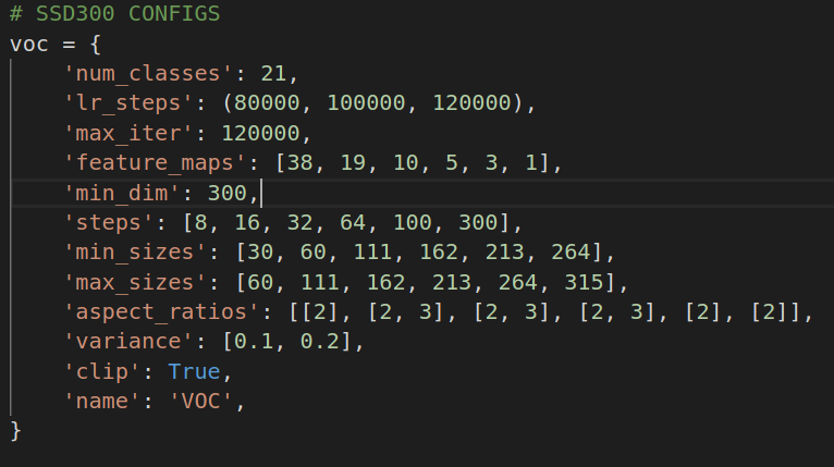
其中

    'min_sizes': [30, 60, 111, 162, 213, 264],      'max_sizes': [60, 111, 162, 213, 264, 315],      'aspect_ratios': [[2], [2, 3], [2, 3], [2, 3], [2], [2]],

用以计算每一个feature map的default box. 这里配置文件的定义让人稍微有点糊涂. min_size/max_size都是用于宽高比为1的box的预测.[2]用于预测宽高比为2:1和1:2的box.

    def forward(self):          mean = []          for k, f in enumerate(self.feature_maps):  #config.py中'feature_maps': [38, 19, 10, 5, 3, 1]              for i, j in product(range(f), repeat=2):                  f_k = self.image_size / self.steps[k]  #基本上除下来和feature_map size类似. 这里直接用f替代f_k区别不大                  # unit center x,y            # 每个feature_map cell的中心                  cx = (j + 0.5) / f_k                  cy = (i + 0.5) / f_k                    # aspect_ratio: 1                  # rel size: min_size                  s_k = self.min_sizes[k]/self.image_size  #min_sizes预测一个宽高比为1的shape                  mean += [cx, cy, s_k, s_k]                    # aspect_ratio: 1                  # rel size: sqrt(s_k * s_(k+1))                  s_k_prime = sqrt(s_k * (self.max_sizes[k]/self.image_size)) #max_size负责预测一个宽高比为1的shape                  mean += [cx, cy, s_k_prime, s_k_prime]                    # rest of aspect ratios #                  for ar in self.aspect_ratios[k]:         #比如对[2,3]则预测4个shape,1;2,2:1,1:3,3:1                      mean += [cx, cy, s_k*sqrt(ar), s_k/sqrt(ar)]                      mean += [cx, cy, s_k/sqrt(ar), s_k*sqrt(ar)]

比如对38 x 38这个feature map的第一个cell,共计算出4个default box.前两个参数是box中点,后面是宽,高.都是相对原图的比例.

tensor([[0.0133, 0.0133, 0.1000, 0.1000],          [0.0133, 0.0133, 0.1414, 0.1414],          [0.0133, 0.0133, 0.1414, 0.0707],          [0.0133, 0.0133, 0.0707, 0.1414]])

预测框生成

feature_map卷积后的tensor含义

每一个feature_map卷积后可得一个m x m x 4的tensor.其中4是(t_x,t_y,t_w,t_h),这时候我们需要用这些数在default box的基础上去得到我们的预测框的坐标.可以认为神经网络预测得到的是相对参考框的偏移. 这也是所谓的把坐标预测当做回归问题的含义.box=anchor_box x 形变矩阵,我们回归的就是这个形变矩阵的参数,即(t_x,t_y,t_w,t_h)
即

               b_center_x = t_x *prior_variance[0]* p_width + p_center_x                 b_center_y = t_y *prior_variance[1] * p_height + p_center_y                 b_width = exp(prior_variance[2] * t_w) * p_width                 b_height = exp(prior_variance[3] * t_h) * p_height  或者                   b_center_x = t_x * p_width + p_center_x                 b_center_y = t_y * p_height + p_center_y                 b_width = exp(t_w) * p_width                 b_height = exp(t_h) * p_height  

其中p_*代表的是default box. b_*才是我们最终预测的box的坐标.

这时候我们得到了很多很多(8732)个box.我们要从这些box中筛选出我们最终给出的box.
伪代码为

for every conv box:      for every class :          if class_prob < theshold:              continue          predict_box = decode(convbox)            nms(predict_box) #去除非常接近的框

代码实现

detection.py

class Detect(Function):          def forward(self, loc_data, conf_data, prior_data):          ##loc_data [batch,8732,4]          ##conf_data [batch,8732,1+class]          ##prior_data [8732,4]            num = loc_data.size(0)  # batch size          num_priors = prior_data.size(0)          output = torch.zeros(num, self.num_classes, self.top_k, 5)          conf_preds = conf_data.view(num, num_priors,                                      self.num_classes).transpose(2, 1)            # Decode predictions into bboxes.          for i in range(num):              decoded_boxes = decode(loc_data[i], prior_data, self.variance)              # For each class, perform nms              conf_scores = conf_preds[i].clone()                for cl in range(1, self.num_classes):                  c_mask = conf_scores[cl].gt(self.conf_thresh)                  scores = conf_scores[cl][c_mask]                  if scores.size(0) == 0:                      continue                  l_mask = c_mask.unsqueeze(1).expand_as(decoded_boxes)                  boxes = decoded_boxes[l_mask].view(-1, 4)                  # idx of highest scoring and non-overlapping boxes per class                  ids, count = nms(boxes, scores, self.nms_thresh, self.top_k)                  output[i, cl, :count] =                       torch.cat((scores[ids[:count]].unsqueeze(1),                                 boxes[ids[:count]]), 1)          flt = output.contiguous().view(num, -1, 5)          _, idx = flt[:, :, 0].sort(1, descending=True)          _, rank = idx.sort(1)          flt[(rank < self.top_k).unsqueeze(-1).expand_as(flt)].fill_(0)          return output      

具体的核心逻辑在box_utils.py

• decode 用于根据卷积结果计算box坐标

def decode(loc, priors, variances):      boxes = torch.cat((          priors[:, :2] + loc[:, :2] * variances[0] * priors[:, 2:],          priors[:, 2:] * torch.exp(loc[:, 2:] * variances[1])), 1)      boxes[:, :2] -= boxes[:, 2:] / 2      boxes[:, 2:] += boxes[:, :2]      return boxes

这里做了一个center_x,center_y, w, h -> xmin, ymin, xmax, ymax的转换.

    boxes[:, :2] -= boxes[:, 2:] / 2      boxes[:, 2:] += boxes[:, :2]

返回的已经是(xmin, ymin, xmax, ymax)的形式来表示box了.

• nms 如果两个框的overlap超过0.5,则认为框的是同一个物体,只保留概率更高的框

def nms(boxes, scores, overlap=0.5, top_k=200):      """Apply non-maximum suppression at test time to avoid detecting too many      overlapping bounding boxes for a given object.      Args:          boxes: (tensor) The location preds for the img, Shape: [num_priors,4].          scores: (tensor) The class predscores for the img, Shape:[num_priors].          overlap: (float) The overlap thresh for suppressing unnecessary boxes.          top_k: (int) The Maximum number of box preds to consider.      Return:          The indices of the kept boxes with respect to num_priors.      """        keep = scores.new(scores.size(0)).zero_().long()      if boxes.numel() == 0:          return keep      x1 = boxes[:, 0]      y1 = boxes[:, 1]      x2 = boxes[:, 2]      y2 = boxes[:, 3]      area = torch.mul(x2 - x1, y2 - y1)      v, idx = scores.sort(0)  # sort in ascending order      # I = I[v >= 0.01]      idx = idx[-top_k:]  # indices of the top-k largest vals      xx1 = boxes.new()      yy1 = boxes.new()      xx2 = boxes.new()      yy2 = boxes.new()      w = boxes.new()      h = boxes.new()        # keep = torch.Tensor()      count = 0      while idx.numel() > 0:          i = idx[-1]  # index of current largest val          # keep.append(i)          keep[count] = i          count += 1          if idx.size(0) == 1:              break          idx = idx[:-1]  # remove kept element from view          # load bboxes of next highest vals          torch.index_select(x1, 0, idx, out=xx1)          torch.index_select(y1, 0, idx, out=yy1)          torch.index_select(x2, 0, idx, out=xx2)          torch.index_select(y2, 0, idx, out=yy2)          # store element-wise max with next highest score          xx1 = torch.clamp(xx1, min=x1[i])          yy1 = torch.clamp(yy1, min=y1[i])          xx2 = torch.clamp(xx2, max=x2[i])          yy2 = torch.clamp(yy2, max=y2[i])          w.resize_as_(xx2)          h.resize_as_(yy2)          w = xx2 - xx1          h = yy2 - yy1          # check sizes of xx1 and xx2.. after each iteration          w = torch.clamp(w, min=0.0)          h = torch.clamp(h, min=0.0)          inter = w*h          # IoU = i / (area(a) + area(b) - i)          rem_areas = torch.index_select(area, 0, idx)  # load remaining areas)          union = (rem_areas - inter) + area[i]          IoU = inter/union  # store result in iou          # keep only elements with an IoU <= overlap          idx = idx[IoU.le(overlap)]      return keep, count

以上就是有关ssd网络结构以及每一层的输出的含义.这些已经足够我们了解推理过程了.即给定一个图,模型如何预测出box的位置.后面我们将继续关注训练的过程.

loss计算

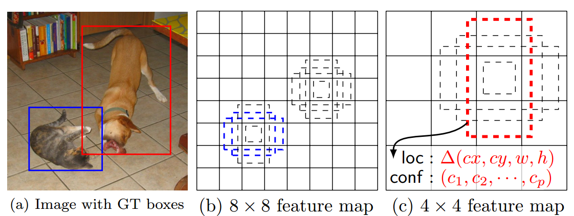
第一个要解决的问题就是box匹配的问题.即每一次训练,怎样的预测框算是预测对了?我们需要计算这些模型认为的预测对了的box和真正的ground truth box之间的差异.

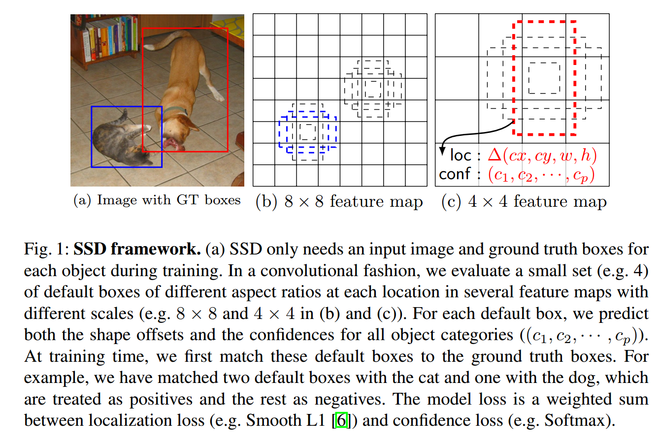
如上所示,猫的ground truth box匹配了2个default box,狗的ground truth box匹配了1个default box.

匹配策略

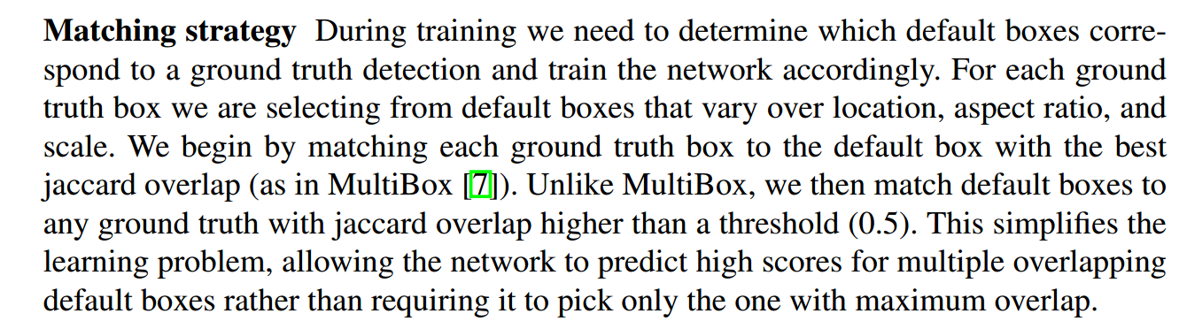
匹配策略是

• 把gt box朝着prior box做匹配,和gt box的IOU最高的prior box被选为正样本
• 任意和gt box的IOU大于0.5的也被选为正样本
  有一个问题困扰了我好久，第二步不是包含第一步吗,直到某天豁然开朗，可能所有的prior box与gt box的iou都<阈值，第一步就是为了保证至少有一个prior box与gt box对应

box_utils.py

def match(threshold, truths, priors, variances, labels, loc_t, conf_t, idx):      # jaccard index     #[objects_num,priorbox_num]      overlaps = jaccard(          truths,          point_form(priors)      )      # (Bipartite Matching)      # [num_objects,1] best prior for each ground truth      best_prior_overlap, best_prior_idx = overlaps.max(1, keepdim=True) #返回每行的最大值,即哪个priorbox与当前obj gt box的IOU最大      # [1,num_priors] best ground truth for each prior      best_truth_overlap, best_truth_idx = overlaps.max(0, keepdim=True) #返回每列的最大值,即哪个obj gt box与当前prior box的IOU最大      best_truth_idx.squeeze_(0) #best_truth_idx的shape是[1,num_priors],去掉第0维度将shape变为[num_priors]      best_truth_overlap.squeeze_(0) #同上      best_prior_idx.squeeze_(1) #best_prior_idx的shape是[num_objects,1],去掉第一维度变为[num_objects]      best_prior_overlap.squeeze_(1)      best_truth_overlap.index_fill_(0, best_prior_idx, 2)  # ensure best prior #把best_truth_overlap第0维度best_prior_idx位置的值的替换为2,以使其肯定>theshold      # TODO refactor: index  best_prior_idx with long tensor      # ensure every gt matches with its prior of max overlap      for j in range(best_prior_idx.size(0)):          best_truth_idx[best_prior_idx[j]] = j      matches = truths[best_truth_idx]          # Shape: [num_priors,4]      conf = labels[best_truth_idx] + 1         # Shape: [num_priors]      conf[best_truth_overlap < threshold] = 0  # label as background      loc = encode(matches, priors, variances)      loc_t[idx] = loc    # [num_priors,4] encoded offsets to learn      conf_t[idx] = conf  # [num_priors] top class label for each prior 

这里的逻辑实际上是有点绕的.给个具体的例子会更好滴帮助你理解.
我们假设一张图片里有2个object.那就有2个gt box,假设计算出3个(实际是8732个)prior box.计算每个gt box和每个prior box的iou即得到一个两行三列的overlaps.

import torch  #假设一幅图里有2个obj,预测出3个box,其iou如overlaps所示  truths = torch.Tensor([[1,2,3,4],[5,6,7,8]]) #2个gtbox 每个box坐标由四个值确定  labels = torch.Tensor([[5],[6]])#2个obj分别属于类别5,类别6  overlaps = torch.Tensor([[0.1,0.4,0.3],[0.5,0.2,0.6]])  #overlaps = torch.Tensor([[0.9,0.9,0.9],[0.8,0.8,0.8]])    best_prior_overlap, best_prior_idx = overlaps.max(1, keepdim=True) #[2,1]  #print(best_prior_overlap)  #print(best_prior_idx) #与目标gt box iou最大的prior box 下标    best_truth_overlap, best_truth_idx = overlaps.max(0, keepdim=True) #返回每列的最大值,即哪个obj gt box与当前prior box的IOU最大  #print(best_truth_overlap) #[1,3]  #print(best_truth_idx) #与prior box iou最大的gt box 下标    best_truth_idx.squeeze_(0) #best_truth_idx的shape是[1,num_priors],去掉第0维度将shape变为[num_priors]  best_truth_overlap.squeeze_(0) #同上    best_prior_idx.squeeze_(1) #best_prior_idx的shape是[num_objects,1],去掉第一维度变为[num_objects]  best_prior_overlap.squeeze_(1)    print(best_prior_idx)  print(best_truth_idx)    #把和gt box的iou最大的prior box的iou设置为2(只要大于阈值就可以了),以确保这个prior box一定会被保留下来.  best_truth_overlap.index_fill_(0, best_prior_idx, 2)    #比如所有的prior box都和gt box1的iou=0.9,prior box2和gt box2的iou=0.8.  我们要确保prior box2被匹配到gt box2而不是gt box1.  #把overlaps = torch.Tensor([[0.9,0.9,0.9],[0.8,0.8,0.8]])试试就知道了  for j in range(best_prior_idx.size(0)):      print(j)      best_truth_idx[best_prior_idx[j]] = j    print(best_truth_idx)    matches = truths[best_truth_idx]  #[3,4] 列代表每一个对应的gt box的坐标  print(matches)    print(best_truth_overlap)    conf = labels[best_truth_idx] + 1 #[3,1]每一列代表当前prior box对应的gt box的类别  print(conf.shape)  #conf[best_truth_overlap < threshold] = 0  #过滤掉iou太低的,标记为background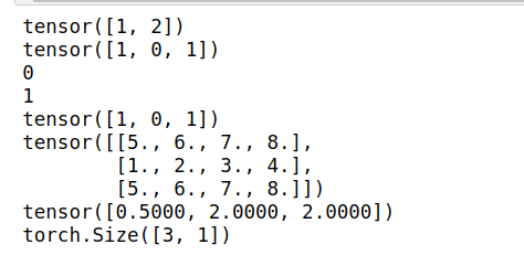

至此,我们得到了matches,即对每一个prior box都找到了其对应的gt box.也得到了conf.即prior box归属的类别.如果iou过低的,类别就被标记为background.

接下来

def encode(matched, priors, variances):      # dist b/t match center and prior's center      g_cxcy = (matched[:, :2] + matched[:, 2:])/2 - priors[:, :2]      # encode variance      g_cxcy /= (variances[0] * priors[:, 2:])      # match wh / prior wh      g_wh = (matched[:, 2:] - matched[:, :2]) / priors[:, 2:]      g_wh = torch.log(g_wh) / variances[1]      # return target for smooth_l1_loss      return torch.cat([g_cxcy, g_wh], 1)  # [num_priors,4]  

我们比较prior box和其对应的gt box的差异.注意这里的matched的格式是(lefttop_x,lefttop_y,rightbottom_x,rightbottom_y).
所以这里得到的其实是gt box和prior box之间的偏移.

计算loss

对于所有的prior box而言,一共可以分为三种类型

• 正样本
• loss排名靠前的xx个负样本
• 其余负样本
  其中正样本即:与ground truth box的iou超过阈值或者iou最大的prior box.
  负样本:正样本之外的prior box.

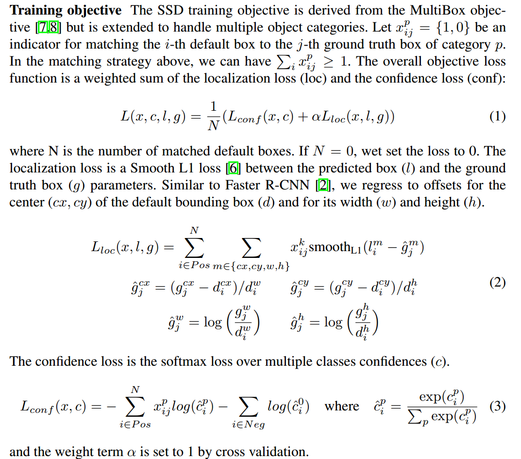
损失函数分为2部分,一部分是坐标偏移的损失,一部分是类别信息的损失.

在计算loc损失的时候,只考虑正样本. 在计算conf损失的时候,即考虑正样本又考虑负样本.并且保持负样本:正样本=3:1.

代码实现在:
multibox_loss.py

class MultiBoxLoss(nn.Module):      def forward(self, predictions, targets):        

伪代码可以表述为

#根据匹配策略得到每个prior box对应的gt box  #根据iou筛选出positive prior box  #计算conf loss  #筛选出loss靠前的xx个negative prior box.保证neg:pos=3:1  #计算交叉熵  #归一化处理

• 坐标偏移的loss

        pos_idx = pos.unsqueeze(pos.dim()).expand_as(loc_data)          loc_p = loc_data[pos_idx].view(-1, 4)  #预测得到的偏移量          loc_t = loc_t[pos_idx].view(-1, 4)     #真实的偏移量          loss_l = F.smooth_l1_loss(loc_p, loc_t, size_average=False)  #我们回归的就是相对default box的偏移

用smooth_l1_loss. 代码比较简单,不多讲了.

Hard negative mining
在匹配default box和gt box以后,必然是有大量的default box是没有匹配上的.即只有少量正样本,有大量负样本.对每个default box,我们按照confidence loss从高到低排序.我们只取排在前列的一些default box去计算loss,使得负样本:正样本在3:1. 这样可以使得模型更加快地优化,训练更稳定.

关于目标检测中的样本不平衡可以参考https://zhuanlan.zhihu.com/p/60612064

简单滴说就是,负样本使得我们学到背景信息,正样本使得我们学到目标信息.所以二者都需要,并且保持一个合适比例.论文里用的是3:1.
对应代码即MultiBoxLoss.negpos_ratio

        # Compute max conf across batch for hard negative mining          batch_conf = conf_data.view(-1, self.num_classes)  #[batch*8732,21]          loss_c = log_sum_exp(batch_conf) - batch_conf.gather(1, conf_t.view(-1, 1)) #conf_t的列方向是类别信息            # Hard Negative Mining          loss_c[pos] = 0  # filter out pos boxes for now          loss_c = loss_c.view(num, -1)          _, loss_idx = loss_c.sort(1, descending=True)          _, idx_rank = loss_idx.sort(1)          num_pos = pos.long().sum(1, keepdim=True)          num_neg = torch.clamp(self.negpos_ratio*num_pos, max=pos.size(1)-1)          #得到负样本的index          neg = idx_rank < num_neg.expand_as(idx_rank)

这时候的loss还不是网络的conf loss,并不是论文里的l_conf.

def log_sum_exp(x):      """Utility function for computing log_sum_exp while determining      This will be used to determine unaveraged confidence loss across      all examples in a batch.      Args:          x (Variable(tensor)): conf_preds from conf layers      """      x_max = x.data.max()      return torch.log(torch.sum(torch.exp(x-x_max), 1, keepdim=True)) + x_max

这里用到了一个trick.参考https://github.com/amdegroot/ssd.pytorch/issues/203,https://stackoverflow.com/questions/42599498/numercially-stable-softmax
为了避免e的n次幂太大或者太小而无法计算,常常在计算softmax时使用这个trick.

这个函数严重影响了我对loss_c的理解,实际上,你可以把上述函数中的x_max移除.那这个函数
那么loss_c就变为了

loss_c = torch.log(torch.sum(torch.exp(batch_conf), 1, keepdim=True)) - batch_conf.gather(1, conf_t.view(-1, 1))

就好理解多了.

conf_t的列方向是相应的label的index. batch_conf.gather(1, conf_t.view(-1, 1))得到一个[batch*8732,1]的tensor,即只保留prior box对应的label的概率预测信息.

那总体的loss即为所有类别的loss之和减去这个prior box应该负责的label的loss.

得到loss_c以后,我们去得到正样本/负样本的index

        # 选出loss最大的一些负样本 负样本:正样本=3:1          # Hard Negative Mining          loss_c = loss_c.view(num, -1) #[batch,8732]          loss_c[pos] = 0  # filter out pos boxes for now          _, loss_idx = loss_c.sort(1, descending=True)  #对每张图的priorbox的conf loss逆序排序          print(_[0,:],loss_idx[0]) #[batch,8732] 每一列的值为prior box的index          _, idx_rank = loss_idx.sort(1)          print(_[0,:],idx_rank[0,:])  #[batch,8732] 每一列的值为prior box在loss_idx的位置.我们要选取前loss_idx中的前xx个.(xx=3倍负样本)          num_pos = pos.long().sum(1, keepdim=True)          print(num_pos) #[batch,1] 列的值为每张图的正样本数量          #求得负样本的数量,3倍正样本,如果3倍正样本>全部prior box,则设置负样本数量为prior box数量          num_neg = torch.clamp(self.negpos_ratio*num_pos, max=pos.size(1)-1)          print(num_neg)          #选出loss排名最靠前的num_neg个负样本          neg = idx_rank < num_neg.expand_as(idx_rank)          print(neg)  

至此,我们就得到了正负样本的下标.接下来就可以计算预测值与真值的差异了.

        loss_c = F.cross_entropy(conf_p, targets_weighted, size_average=False)            # Sum of losses: L(x,c,l,g) = (Lconf(x, c) + αLloc(x,l,g)) / N            N = num_pos.data.sum()          loss_l /= N          loss_c /= N          return loss_l, loss_c  

用交叉熵衡量loss. 最后除以正样本的数量,做归一化处理.
https://pytorch.org/docs/stable/nn.html#torch.nn.CrossEntropyLoss

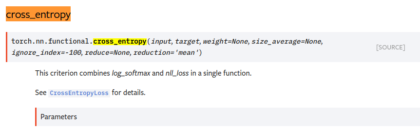
在计算loss前,不需要手动softmax转换成概率值了.

训练

前面已经实现了网络结构创建,loss计算.接下来就可以实现训练了.
实现在train.py
精简后的主要逻辑如下:

    ssd_net = build_ssd('train', cfg['min_dim'], cfg['num_classes'])      net = ssd_net        optimizer = optim.SGD(net.parameters(), lr=args.lr, momentum=args.momentum,                            weight_decay=args.weight_decay)      criterion = MultiBoxLoss(cfg['num_classes'], 0.5, True, 0, True, 3, 0.5,                               False, args.cuda)        for iteration in range(args.start_iter, cfg['max_iter']):          # load train data          images, targets = next(batch_iterator)            # forward          out = net(images)            # backprop          optimizer.zero_grad()          loss_l, loss_c = criterion(out, targets)          loss = loss_l + loss_c          loss.backward()          optimizer.step()      

即

• 定义网络结构
• 定义损失函数及反向传播求梯度方法
• 加载训练集
• 前向传播得到预测值
• 计算loss
• 反向传播,更新网络权重参数

涉及到的部分torch中函数用法参考:https://www.cnblogs.com/sdu20112013/p/11731741.html