感知機演算法(PLA)程式碼實現
- 2020 年 7 月 22 日
- 筆記
- Machine Learning
目錄
1. 引言
在這裡主要實現感知機演算法(PLA)的以下幾種情況:
- PLA演算法的原始形式(二分類)
- PLA演算法的對偶形式(二分類)
- PLA演算法的作圖(二維)
- PLA演算法的多分類情況(包括one vs. rest 和one vs. one 兩種情況)
- PLA演算法的sklearn實現
為了方便起見,使用鳶尾花數據集進行PLA演算法的驗證。
2. 載入庫和數據處理
# 載入庫
import numpy as np
import pandas as pd
import matplotlib.pyplot as plt
from sklearn.datasets import load_iris
from sklearn.model_selection import train_test_split
from sklearn.linear_model import Perceptron
import warnings
warnings.filterwarnings("ignore")

# 設置圖形尺寸
plt.rcParams["figure.figsize"] = [14, 7]
plt.rcParams["font.size"] = 14

# 載入鳶尾花數據集
iris_data = load_iris()
xdata = iris_data["data"]
ydata = iris_data["target"]
3. 感知機的原始形式
感知機的詳細原理見我的前一篇部落格
class model_perceptron(object):
    """
    功能:實現感知機演算法
    參數 w:權重,默認都為None
    參數 b:偏置項,默認為0
    參數 alpha:學習率,默認為0.001
    參數 iter_epoch:迭代輪數,默認最大為1000
    """
    def __init__(self, w = None, b = 0, alpha = 0.001, max_iter_epoch = 1000):
        self.w = w
        self.b = b
        self.alpha = alpha
        self.max_iter_epoch = max_iter_epoch

    def linear_model(self, X):
        """功能:實現線性模型"""
        return np.dot(X, self.w) + self.b

    def fit(self, X, y):
        """
        功能:擬合感知機模型
        參數 X:訓練集的輸入數據
        參數 y:訓練集的輸出數據
        """
        # 按訓練集的輸入維度初始化w
        self.w = np.zeros(X.shape[1])
        # 誤分類的樣本就為True
        state = np.sign(self.linear_model(X)) != y
        # 迭代輪數
        total_iter_epoch = 1

        while state.any() and (total_iter_epoch <= self.max_iter_epoch):
            # 使用誤分類點進行權重更新
            self.w += self.alpha * y[state][0] * X[state][0]
            self.b += self.alpha * y[state][0]

            # 狀態更新
            total_iter_epoch += 1
            state = np.sign(self.linear_model(X)) != y

        print(f"fit model_perceptron(alpha = {self.alpha}, max_iter_epoch = {self.max_iter_epoch}, total_iter_epoch = {min(self.max_iter_epoch, total_iter_epoch)})")

    def predict(self, X):
        """
        功能:模型預測
        參數 X:測試集的輸入數據
        """
        return np.sign(self.linear_model(X))

    def score(self, X, y):
        """
        功能:模型評價(準確率)
        參數 X:測試集的輸入數據
        參數 y:測試集的輸出數據
        """
        y_predict = self.predict(X)
        y_score = (y_predict == y).sum() / len(y)

        return y_score
# 二分類的情況(原始形式)/ 數據集的處理與劃分
X = xdata[ydata < 2]
y = ydata[ydata < 2]
y = np.where(y == 0, -1, 1)
xtrain, xtest, ytrain, ytest = train_test_split(X, y)
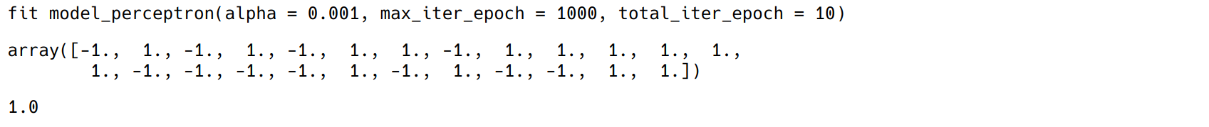
# 原始形式的驗證
ppn = model_perceptron()
ppn.fit(xtrain, ytrain)
ppn.predict(xtest)
ppn.score(xtest, ytest)
結果顯示(由於隨機劃分數據集,運行結果不一定和圖示相同):
4. 感知機的對偶形式
class perceptron_dual(object):
    """
    功能:實現感知機的對偶形式
    參數 beta:每個實例點更新的次數組成的向量
    參數 w:權重,默認都為None
    參數 b:偏置項,默認為0
    參數 alpha:學習率,默認0.001
    參數 max_iter_epoch:最大迭代次數,默認為1000
    """
    def __init__(self, alpha = 0.001, max_iter_epoch = 1000):
        self.beta = None
        self.w = None
        self.b = 0
        self.alpha = alpha
        self.max_iter_epoch = max_iter_epoch

    def fit(self, X, y):
        # 實例點的數量
        xnum = X.shape[0]
        # 初始化
        self.beta = np.zeros(xnum)

        # gram矩陣
        gram = np.dot(X, X.T)

        # 迭代條件
        state = y*((self.beta * y * gram).sum(axis = 1) + self.b) <= 0
        iter_epoch = 1

        while state.any() and (iter_epoch <= self.max_iter_epoch):
            nx = X[state][0]
            ny = y[state][0]
            index = (X == nx).argmax()
            self.beta[index] += self.alpha
            self.b += ny

            # 更新條件
            iter_epoch += 1
            state = y*((self.beta * y * gram).sum(axis = 1) + self.b) <= 0

        # 通過beta計算出w
        self.w = ((self.beta * y).reshape(-1, 1) * X).sum(axis = 0)
        print(f"fit perceptron_dual(alpha = {self.alpha}, total_iter_epoch = {min(self.max_iter_epoch, iter_epoch)})")


    def predict(self, X):
        """
        功能:模型預測
        參數 X:測試集的輸入數據
        """
        y_predict = np.sign(X @ self.w  + self.b)
        return y_predict

    def score(self, X, y):
        """
        功能:模型評價(準確率)
        參數 X:測試集的輸入數據
        參數 y:測試集的輸出數據
        """
        y_score = (self.predict(X) == y).sum() / len(y)

        return y_score
# 二分類的情況(對偶形式)/ 數據集的處理與劃分
X = xdata[ydata < 2]
y = ydata[ydata < 2]
y = np.where(y == 0, -1, 1)
xtrain, xtest, ytrain, ytest = train_test_split(X, y)
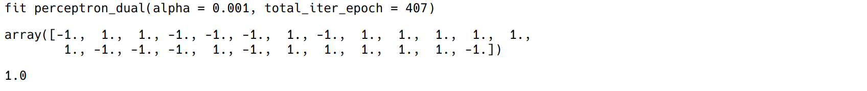
# 對偶形式驗證
ppn = perceptron_dual()
ppn.fit(xtrain, ytrain)
ppn.predict(xtest)
ppn.score(xtest, ytest)
結果顯示(由於隨機劃分數據集,運行結果不一定和圖示相同):
5. 多分類情況—one vs. rest
假設有k個類別,ovr策略是生成k個分類器,最後選取概率最大的預測結果
class perceptron_ovr(object):
    """
    功能:實現感知機的多分類情形(採用one vs. rest策略)
    參數 w:權重,默認都為None
    參數 b:偏置項,默認為0
    參數 alpha:學習率,默認0.001
    參數 max_iter_epoch:最大迭代次數,默認為1000
    """
    def __init__(self, alpha = 0.001, max_iter_epoch = 1000):
        self.w = None
        self.b = None
        self.alpha = alpha
        self.max_iter_epoch = max_iter_epoch

    def linear_model(self, X):
        """功能:實現線性模型"""
        return np.dot(self.w, X.T) + self.b

    def fit(self, X, y):
        """
        功能:擬合感知機模型
        參數 X:訓練集的輸入數據
        參數 y:訓練集的輸出數據
        """
        # 生成各分類器對應的標記
        self.y_class = np.unique(y)
        y_ovr = np.vstack([np.where(y == i, 1, -1) for i in self.y_class])

        # 初始化w, b
        self.w = np.zeros([self.y_class.shape[0], X.shape[1]])
        self.b = np.zeros([self.y_class.shape[0], 1])

        # 擬合各分類器,並更新相應維度的w和b
        for index in range(self.y_class.shape[0]):
            ppn = model_perceptron(alpha = self.alpha, max_iter_epoch = self.max_iter_epoch)
            ppn.fit(X, y_ovr[index])
            self.w[index] = ppn.w
            self.b[index] = ppn.b

    def predict(self, X):
        """
        功能:模型預測
        參數 X:測試集的輸入數據
        """
        # 值越大,說明第i維的分類器將該點分得越開,即屬於該分類器的概率值越大
        y_predict = self.linear_model(X).argmax(axis = 0)

        # 還原原數據集的標籤
        for index in range(self.y_class.shape[0]):
            y_predict = np.where(y_predict == index, self.y_class[index], y_predict)

        return y_predict

    def score(self, X, y):
        """
        功能:模型評價(準確率)
        參數 X:測試集的輸入數據
        參數 y:測試集的輸出數據
        """
        y_score = (self.predict(X) == y).sum()/len(y)
        return y_score
# 多分類數據集處理
xtrain, xtest, ytrain, ytest = train_test_split(xdata, ydata)
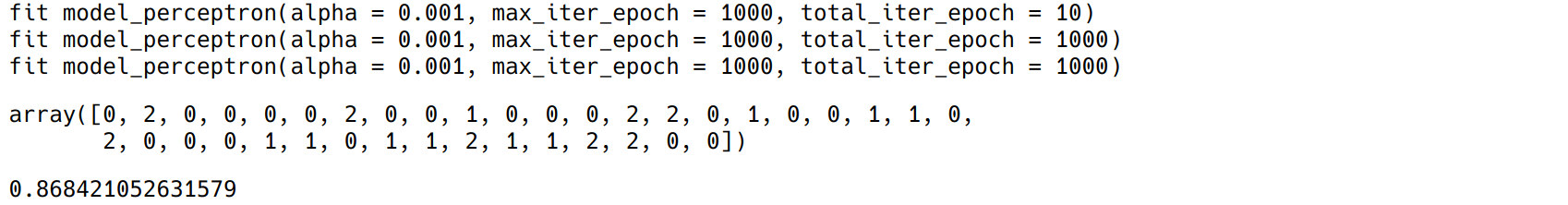
# one vs. rest的驗證
ppn = perceptron_ovr()
ppn.fit(xtrain, ytrain)
ppn.predict(xtest)
ppn.score(xtest, ytest)
結果顯示(由於隨機劃分數據集,運行結果不一定和圖示相同):
6. 多分類情況—one vs. one
假設有k個類別,生成k(k-1)/2個二分類器,最後通過多數投票來選取預測結果
from itertools import combinations

class perceptron_ovo(object):
    """
    功能:實現感知機的多分類情形(採用one vs. one策略)
    參數 w:權重,默認都為None
    參數 b:偏置項,默認為0
    參數 alpha:學習率,默認0.001
    參數 max_iter_epoch:最大迭代次數,默認為1000
    """
    def __init__(self, alpha = 0.001, max_iter_epoch = 1000):
        self.w = None
        self.b = None
        self.alpha = alpha
        self.max_iter_epoch = max_iter_epoch

    def linear_model(self, X):
        """功能:實現線性模型"""
        return np.dot(self.w, X.T) + self.b

    def fit(self, X, y):
        """
        功能:擬合感知機模型
        參數 X:訓練集的輸入數據
        參數 y:訓練集的輸出數據
        """
        # 生成各分類器對應的標記(使用排列組合)
        self.y_class = np.unique(y)
        self.y_combine = [i for i in combinations(self.y_class, 2)]

        # 初始化w和b
        clf_num = len(self.y_combine)
        self.w = np.zeros([clf_num, X.shape[1]])
        self.b = np.zeros([clf_num, 1])

        for index, label in enumerate(self.y_combine):
            # 根據各分類器的標籤選取數據集
            cond = pd.Series(y).isin(pd.Series(label))
            xdata, ydata = X[cond], y[cond]
            ydata = np.where(ydata == label[0], 1, -1)

            # 擬合各分類器,並更新相應維度的w和b
            ppn = model_perceptron(alpha = self.alpha, max_iter_epoch = self.max_iter_epoch)
            ppn.fit(xdata, ydata)
            self.w[index] = ppn.w
            self.b[index] = ppn.b

    def voting(self, y):
        """
        功能:投票
        參數 y:各分類器的預測結果,接受的是元組如(1, 1, 2)
        """
        # 統計分類器預測結果的出現次數
        y_count = np.unique(np.array(y), return_counts = True)
        # 返回出現次數最大的結果位置索引
        max_index = y_count[1].argmax()
        # 返回某個實例投票後的結果
        y_predict = y_count[0][max_index]

        return y_predict


    def predict(self, X):
        """
        功能:模型預測
        參數 X:測試集的輸入數據
        """
        # 預測結果
        y_predict = np.sign(self.linear_model(X))
        # 還原標籤(根據排列組合的標籤)
        for index, label in enumerate(self.y_combine):
            y_predict[index] = np.where(y_predict[index] == 1, label[0], label[1])

        # 列為某一個實例的預測結果,打包用於之後的投票
        predict_zip = zip(*(i.reshape(-1) for i in np.vsplit(y_predict, self.y_class.shape[0])))
        # 投票得到預測結果
        y_predict = list(map(lambda x: self.voting(x), list(predict_zip)))

        return np.array(y_predict)

    def score(self, X, y):
        """
        功能:模型評價(準確率)
        參數 X:測試集的輸入數據
        參數 y:測試集的輸出數據
        """
        y_predict = self.predict(X)
        y_score = (y_predict == y).sum() / len(y)

        return y_score
# 多分類數據集處理
xtrain, xtest, ytrain, ytest = train_test_split(xdata, ydata)

# one vs. one的驗證
ppn = perceptron_ovo()
ppn.fit(xtrain, ytrain)
ppn.predict(xtest)
ppn.score(xtest, ytest)
結果顯示(由於隨機劃分數據集,運行結果不一定和圖示相同):

準確率一般比one vs. rest要高,但是生成的分類器多
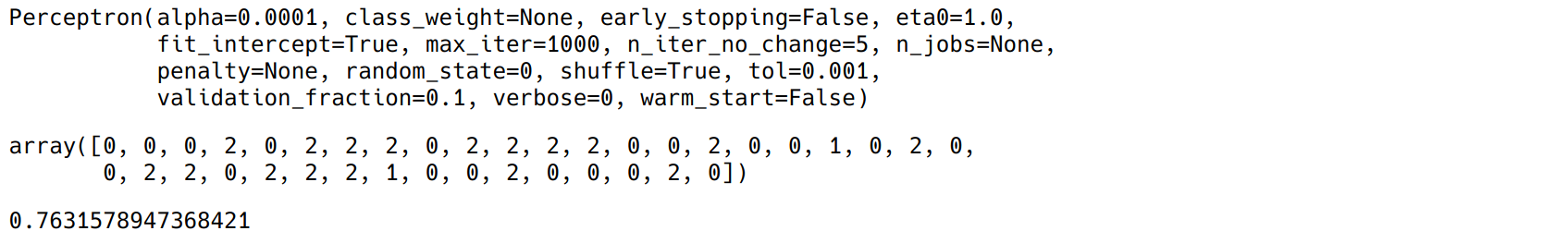
7. sklearn實現
主要使用sklearn中的Perceptron模組,其中可以實現多分類的情況(默認採用one vs. rest)
from sklearn.linear_model import Perceptron

xtrain, xtest, ytrain, ytest = train_test_split(xdata, ydata)
ppn = Perceptron(max_iter = 1000)
ppn.fit(xtrain, ytrain)
ppn.predict(xtest)
ppn.score(xtest, ytest)
結果顯示:
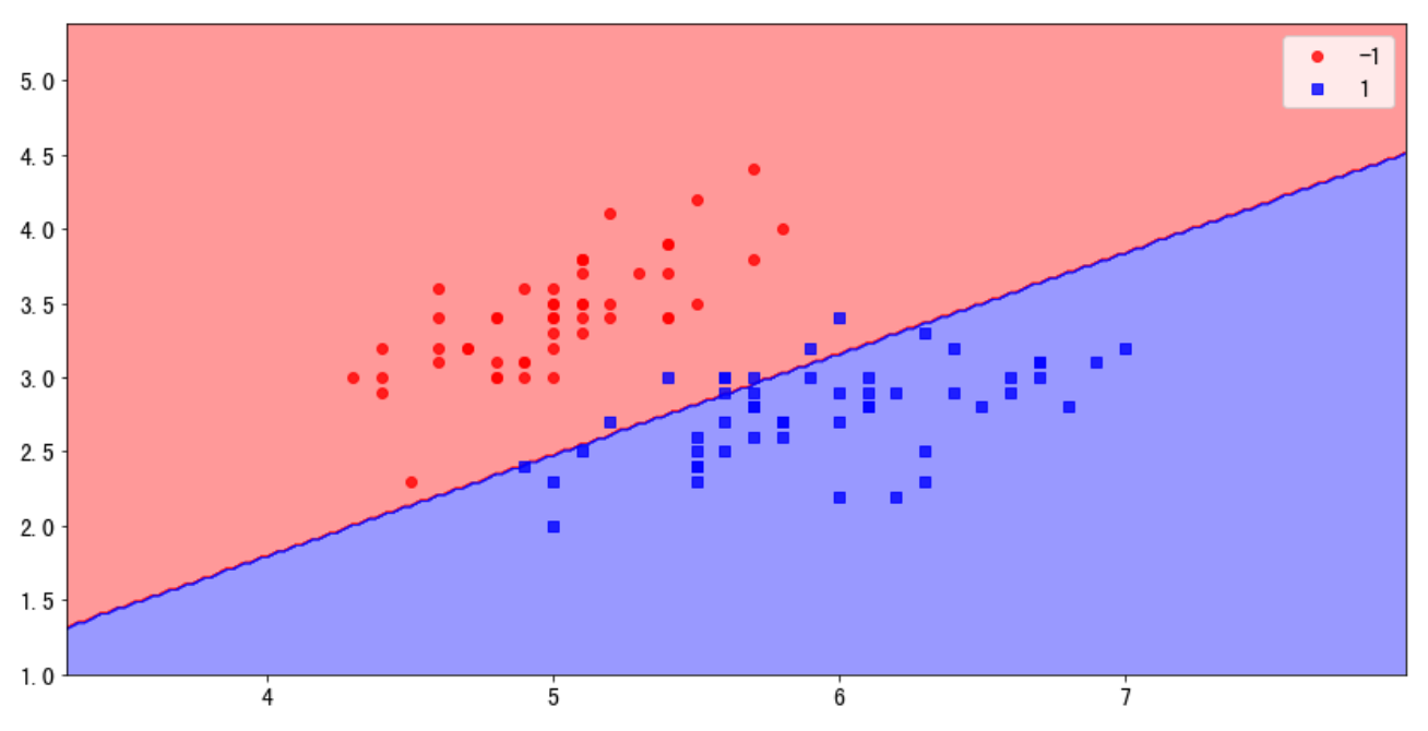
8. 感知機演算法的作圖
from matplotlib.colors import ListedColormap

def decision_plot(X, Y, clf, test_idx = None, resolution = 0.02):
    """
    功能:畫分類器的決策圖
    參數 X:輸入實例
    參數 Y:實例標記
    參數 clf:分類器
    參數 test_idx:測試集的index
    參數 resolution:np.arange的間隔大小
    """
    # 標記和顏色設置
    markers = ['o', 's', 'x', '^', '>']
    colors = ('red', 'blue', 'lightgreen', 'gray', 'cyan')
    cmap = ListedColormap(colors[:len(np.unique(Y))])

    # 圖形範圍
    xmin, xmax = X[:, 0].min() - 1, X[:, 0].max() + 1
    ymin, ymax = X[:, 1].min() - 1, X[:, 1].max() + 1
    x = np.arange(xmin, xmax, resolution)
    y = np.arange(ymin, ymax, resolution)

    # 網格
    nx, ny = np.meshgrid(x, y)

    # 數據合併
    xdata = np.c_[nx.reshape(-1), ny.reshape(-1)]

    # 分類器預測
    z = clf.predict(xdata)
    z = z.reshape(nx.shape)

    # 作區域圖
    plt.contourf(nx, ny, z, alpha = 0.4, cmap = cmap)
    plt.xlim(nx.min(), nx.max())
    plt.ylim(ny.min(), ny.max())

    # 畫點
    for index, cl in enumerate(np.unique(Y)):
        plt.scatter(x=X[Y == cl, 0], y=X[Y == cl, 1],
                    alpha=0.8, c = cmap(index),
                    marker=markers[index], label=cl)

    # 突出測試集的點
    if test_idx:
        X_test, y_test = X[test_idx, :], y[test_idx]

        plt.scatter(X_test[:, 0],
                    X_test[:, 1],
                    alpha=0.15,
                    linewidths=2,
                    marker='^',
                    edgecolors='black',
                    facecolors='none',
                    s=55, label='test set')
# 作圖時的數據處理
X = xdata[ydata < 2, :2]
y = ydata[ydata < 2]
y = np.where(y == 0, -1, 1)

xtrain, xtest, ytrain, ytest = train_test_split(X, y)
ppn = model_perceptron()
ppn.fit(xtrain, ytrain)
decision_plot(X, y, ppn)
plt.legend()
結果顯示: