機器學習中的數據準備
數據準備是機器學習中一項非常重要的環節,本文主要對數據準備流程進行簡單的梳理,主要參考了Data Preparation for Machine Learning一書。
數據準備需要進行的工作主要分為以下幾類:
- 數據清理(Data Cleaning)
- 數據轉換(Data Transformation)
- 特徵選擇(Feature Selection)
數據清理
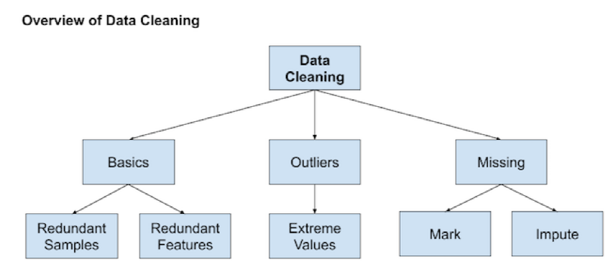
- 刪除冗餘的特徵或樣本
# delete columns with a single unique value
counts = df.nunique()
to_del = [i for i,v in enumerate(counts) if v == 1]
df.drop(to_del, axis=1, inplace=True)

# delete rows of duplicate data from the dataset
df.drop_duplicates(inplace=True)
- 尋找異常點
- 統計學方法
- 若特徵屬於正態分佈$N(\mu,\sigma^2)$,則區間$[\mu-3\sigma,\text{ }\mu+3\sigma]$之外的值可視為異常值
- 若特徵屬於偏態分佈,則定義IQR = 75th quantile – 25th quantile,區間[25th quantile – c*IQR, 75th quantile + c*IQR]之外的值可視為異常值,c通常取1.5或3
- 自動檢測方法
- Local Outlier Factor (LOF):LOF算法原理介紹
# identify outliers in the training dataset
lof = LocalOutlierFactor()
yhat = lof.fit_predict(X_train)
# Method 1: select all rows that are not outliers
mask = yhat != -1
X_train, y_train = X_train[mask, :], y_train[mask]
# Method 2: check LOF score
score = lof.negative_outlier_factor_
X_train, y_train = X_train[score>threshold], y_train[score>threshold]
- Isolation Forest: Isolation Forest算法原理介紹
rng = np.random.RandomState(42)
clf = IsolationForest(max_samples=256,  random_state=rng, contamination='auto')
yhat = clf.fit_predict(X_train)
mask = yhat != -1
X_train, y_train = X_train[mask, :], y_train[mask]
- Local Outlier Factor (LOF):LOF算法原理介紹
- 統計學方法
- 處理缺失值
- 直接刪除有缺失值的數據
- 使用特徵的統計量(Mean, Median, Mode, Constant)進行填充
# define imputer
imputer = SimpleImputer(strategy='mean')
# fit on the training dataset (fit函數僅在訓練數據上使用,防止data leakage)
Xtrans = imputer.fit_transform(X_train)
- 將缺失值單獨標記為一個新的類別,例如’Missing’,適用於類別特徵
- 加入一個新的特徵(二值變量,取值為0或1),來對應某個特徵是否缺失(1: 缺失,0: 正常)。該方法通常和其它缺失值填充方法配合使用
- k-Nearest Neighbour Imputation
pipeline = Pipeline(steps=[('i', KNNImputer(n_neighbors=...)), ('m', RandomForestClassifier())])
# evaluate the model
cv = RepeatedStratifiedKFold(n_splits=10, n_repeats=3, random_state=1)
scores = cross_val_score(pipeline, X, y, scoring='accuracy', cv=cv, n_jobs=-1)
- Iterative Imputation
##############################################################
#1. 對每個缺失值進行初始填充
#2. 根據選定的特徵順序依次對有缺失值的特徵建立預測模型,將其表示為其它特徵的函數,訓練模型並預測該特徵的缺失值,使用預測值更新缺失值
#3. 不斷重複上一步驟進行迭代
##############################################################

# estimator: 使用的預測模型
# imputation_order: 進行缺失值更新和填充的特徵順序
# n_nearest_features: 模型訓練和預測使用的特徵數量
# max_iter: 最大迭代次數
# initial_strategy: 初始填充使用的填充策略
pipeline = Pipeline(steps=[('i', IterativeImputer(estimator=..., max_iter=..., n_nearest_features=..., initial_strategy=..., imputation_order=...)), ('m', RandomForestClassifier())])
# evaluate the model
cv = RepeatedStratifiedKFold(n_splits=10, n_repeats=3, random_state=1)
scores = cross_val_score(pipeline, X, y, scoring='accuracy', cv=cv, n_jobs=-1)
數據轉換

- 數值特徵的尺度變換
- Data Normalization: 將特徵變換到[0,1]之間。$\frac{value – min}{max – min}$, MinMaxScaler()
- Data Standardization: 將特徵均值變為0,標準差變為1。$\frac{value – mean}{standard\_deviation}$, StandardScaler()
- Robust Scale: 類似Data Standardization,但選用較穩健的特徵統計量(median、IQR),減少異常值對特徵統計量的影響。$\frac{value – median}{IQR}$, 其中IQR = 75th quantile – 25th quantile, RobustScaler()
- 數值特徵的分佈變換
- 將特徵轉換為高斯分佈可以增加一些模型的預測準確度
- Power Transform (e.g., $\ln{x},\text{ }\sqrt{x}$): PowerTransformer(method=…),對原始特徵進行尺度變換之後使用該方法有時會比直接使用產生更好效果
- Quantile Transform: 利用cumulative distribution function (CDF)將特徵的分佈直接映射成高斯分佈,QuantileTransformer(output_distribution=‘normal’)
- 特徵離散化,即轉換為類別特徵,主要有下圖所示的三種方法
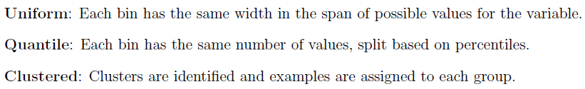
BinsDiscretizer(n_bins=…, encode=…, strategy=…)
- 將特徵轉換為高斯分佈可以增加一些模型的預測準確度
- 類別特徵的編碼
- One-Hot Encode: 如果一個特徵中有$k$個類別,則將該特徵轉換為$k$個新的二值特徵(例如”顏色:紅、黃、綠”變為:”顏色_紅:1、0、0″以及”顏色_黃:0、1、0″以及”顏色_綠:0、0、1″),常用於決策樹模型,例如CART、RandomForest,函數API為OneHotEncoder(drop=None, …);或者將其轉換為$k-1$個新的特徵(例如”顏色:紅、黃、綠”變為:”顏色_黃:0、1、0″以及”顏色_綠:0、0、1″),常用於包含偏差項(i.e., bias term)的模型,例如線性回歸,函數API為OneHotEncoder(drop=『first』, …)
- One-Hot Encode for Top Categories:如果一個特徵中包含的類別較多,則可將one-hot encode限制在出現頻率最高的幾個類別中,例如可將特徵轉換為10個新的二值特徵,這些新特徵對應原特徵中出現頻率最高的10個類別
- Ordinal Encode: 將特徵中的類別按順序編碼為0, 1, 2, …,OrdinalEncoder()
- Frequency Encode:將特徵中的類別編碼為該類別在特徵中出現的頻率或次數
- Mean Encode: 將特徵中的類別編碼為該類別對應的預測量的均值
- Ordered Integer Encode: 根據特徵中每個類別對應的預測量的均值從大到小將類別編碼為0, 1, 2, …
- 特徵工程
- 生成Polynomial Features: PolynomialFeatures(degree=…, interaction_only=…, include_bias=…)
- Deep Feature Synthesis (深度特徵綜合): 可同時處理多個數據表進行轉換 (transformation) 或聚合 (aggregation) 操作,自動生成新的特徵。使用方式可參考自動化特徵工程—Featuretools
- 上述技術有一些也可用於預測量上,例如在預測量上進行Power Transform不僅可以減少預測量的偏度(skewness),使之更接近高斯分佈,還可以起到穩定方差的作用,減弱Heteroscedasticity效應。可使用TransformedTargetRegressor對預測量進行轉換,例如:
# prepare the model with input scaling and power transform
steps = list()
steps.append(('scale', MinMaxScaler(feature_range=(1e-5,1))))
steps.append(('power', PowerTransformer()))
steps.append(('model', HuberRegressor()))
pipeline = Pipeline(steps=steps)
# prepare the model with target power transform
model = TransformedTargetRegressor(regressor=pipeline, transformer=PowerTransformer())
# evaluate model
cv = RepeatedKFold(n_splits=10, n_repeats=3, random_state=1)
scores = cross_val_score(model, X, y, scoring='neg_mean_absolute_error', cv=cv, n_jobs=-1)
- 可使用ColumnTransformer對不同的特徵進行不同的轉換,例如:
# determine categorical and numerical features
numerical_ix = X.select_dtypes(include=['int64', 'float64']).columns
categorical_ix = X.select_dtypes(include=['object', 'bool']).columns
# define the data preparation for the columns
t = [('cat', OneHotEncoder(), categorical_ix), ('num', MinMaxScaler(), numerical_ix)]
col_transform = ColumnTransformer(transformers=t, remainder=...)
# define the data preparation and modeling pipeline
pipeline = Pipeline(steps=[('prep',col_transform), ('m', model)])

特徵選擇
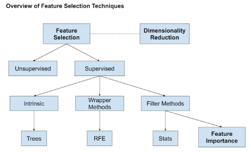
- Filter Methods
- 統計方法
- ${\chi}^2$ Test: 適用於分類問題,只能用於非負特徵(包括類別特徵)的選擇,具體介紹可參考這篇文章中的”4. 處理文本特徵”
SelectKBest(score_func=chi2, k=...)
- Mutual Information: $I(X ; Y)=\int_{Y} \int_{X} p(x, y) \log \left(\frac{p(x, y)}{p(x) p(y)}\right) d x d y,\text{ }I(X ; Y)>=0且僅在X和Y相互獨立時為0$
SelectKBest(score_func=mutual_info_classif, k=...)  #classification
SelectKBest(score_func=mutual_info_regression, k=...)  #regression
- One-Way ANOVA: 適用於分類問題,用於數值特徵的選擇
SelectKBest(score_func=f_classif, k=...)
- Pearson Correlation: 適用於回歸問題,用於數值特徵的選擇
SelectKBest(score_func=f_regression, k=...)
- ${\chi}^2$ Test: 適用於分類問題,只能用於非負特徵(包括類別特徵)的選擇,具體介紹可參考這篇文章中的”4. 處理文本特徵”
- 特徵重要性
- feature importance from model coefficients (model.coef_)
SelectFromModel(estimator=..., max_features=..., threshold=...)
- feature importance from decision trees (model.feature_importances_)
SelectFromModel(estimator=..., max_features=..., threshold=...)
- feature importance from permutation testing: 將一個選定的模型訓練好之後,將訓練集或驗證集上的某一個特徵的值隨機打亂順序,打亂順序前後模型在該數據集上預測能力的變化反映了該特徵的重要程度
### Example 1 ###
model = KNeighborsRegressor()
model.fit(X_train, y_train) # fit the model
# perform permutation importance
results = permutation_importance(model, X_train, y_train, scoring='neg_mean_squared_error')
importance = results.importances_mean  #get importance

### Example 2 ###
model = Ridge(alpha=1e-2).fit(X_train, y_train)
r = permutation_importance(model, X_val, y_val, n_repeats=30, random_state=0)
importance = r.importances_mean
- feature importance from model coefficients (model.coef_)
- 統計方法
- Recursive Feature Elimination (RFE): 對選定的模型進行迭代訓練,每次訓練後根據得到的特徵重要性刪除一些特徵,在此基礎上重新進行訓練
RFE(estimator=..., n_features_to_select=..., step=...)
-
Dimension Reduction: LDA(有監督降維), PCA(無監督降維),算法原理可參考PCA與LDA介紹


