LetNet、Alex、VggNet分析及其pytorch实现
简单分析一下主流的几种神经网络
LeNet
LetNet作为卷积神经网络中的HelloWorld,它的结构及其的简单,1998年由LeCun提出
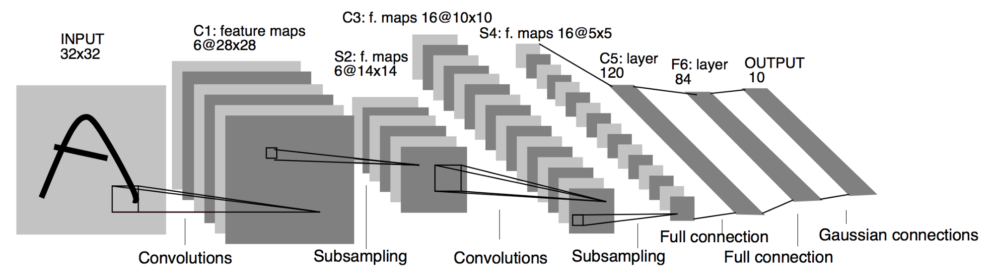
基本过程:
可以看到LeNet-5跟现有的conv->pool->ReLU的套路不同,它使用的方式是conv1->pool->conv2->pool2再接全连接层,但是不变的是,卷积层后紧接池化层的模式依旧不变。
代码:
import torch.nn as nn
import torch


class LeNet(nn.Module):
    def __init__(self):
        super(LeNet, self).__init__()

        layer1 = nn.Sequential()
        # Convolution with 5x5 kernel+2padding:28×28×6
        layer1.add_module('conv1', nn.Conv2d(1, 6, kernel_size=(3, 3), padding=1))
        # Pool with 2x2 average kernel+2 stride:14×14×6
        layer1.add_module('pool1', nn.MaxPool2d(kernel_size=2))
        self.layer1 = layer1

        layer2 = nn.Sequential()
        # Convolution with 5x5 kernel (no pad):10×10×16
        layer2.add_module('conv2', nn.Conv2d(6, 16, kernel_size=(5, 5)))
        # Pool with 2x2 average kernel+2 stride: 5x5×16
        layer2.add_module('pool2', nn.MaxPool2d(kernel_size=2))
        self.layer2 = layer2

        layer3 = nn.Sequential()
        # 5 = ((28/2)-4)/2
        layer3.add_module('fc1', nn.Linear(16 * 5 * 5, 120))
        layer3.add_module('fc2', nn.Linear(120, 84))
        layer3.add_module('fc3', nn.Linear(84, 10))
        self.layer3 = layer3

    def forward(self, x):
        x = self.layer1(x)
        # print(x.size())
        x = self.layer2(x)
        # print(x.size())
        # 展平x
        x = torch.flatten(x, 1)
        x = self.layer3(x)
        return x


# 测试
test_data = torch.rand(1, 1, 28, 28)
model = LeNet()
model(test_data)
输出
tensor([[ 0.0067, -0.0431,  0.1072,  0.1275,  0.0143,  0.0865, -0.0490, -0.0936,
         -0.0315, -0.0367]], grad_fn=<AddmmBackward0>)
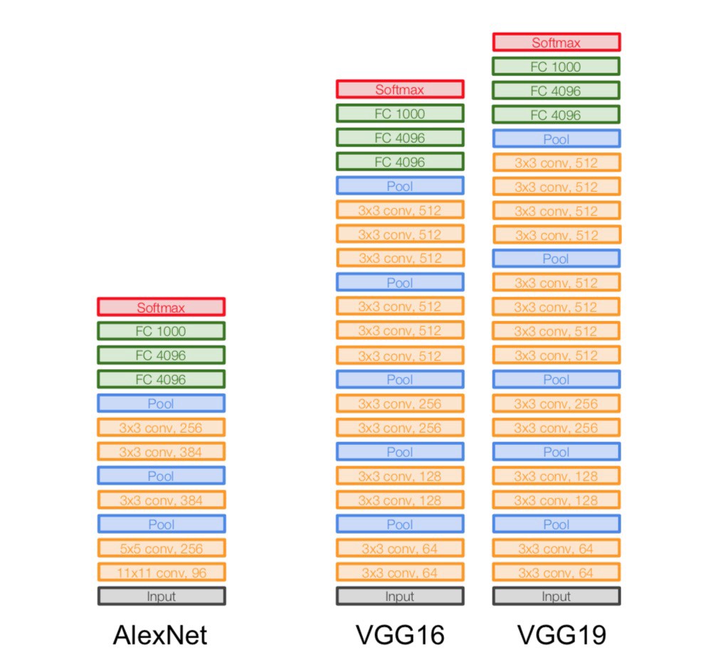
AlexNet
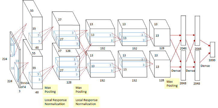
这个图看起来稍微可能有亿点复杂,其实这个是因为当时的GPU计算能力不太行,而Alex又比较复杂,所以Alex使用了两个GPU并行来做运算,现在已经完全可以用一个GPU来代替了。
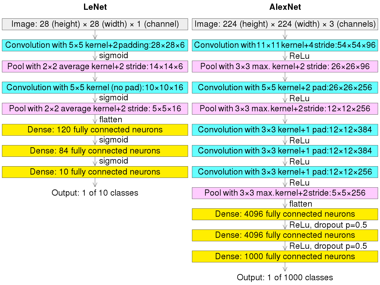
相对于LeNet来说,Alex网络层数更深,同时第一次引入了激活层ReLU,又在全连接层引入了Dropout层防止过拟合。
执行流程图在上面,跟LeNet的执行流程图放在一张图上。
代码:
import torch.nn as nn
import torch


class AlexNet(nn.Module):
    def __init__(self, num_class):
        super(AlexNet, self).__init__()
        self.features = nn.Sequential(
            nn.Conv2d(3, 64, kernel_size=(11, 11), stride=(4, 4)),
            nn.ReLU(True),
            nn.MaxPool2d(kernel_size=3, stride=2),
            nn.Conv2d(64, 192, kernel_size=(5, 5), padding=2),
            nn.ReLU(True),
            nn.MaxPool2d(kernel_size=3, stride=2),
            nn.Conv2d(192, 384, kernel_size=(3, 3), padding=1),
            nn.ReLU(True),
            nn.Conv2d(384, 256, kernel_size=(3, 3), padding=1),
            nn.ReLU(True),
            nn.Conv2d(256, 256, kernel_size=(3, 3), padding=1),
            nn.ReLU(True),
            nn.MaxPool2d(kernel_size=3, stride=2),
        )

        self.classifier = nn.Sequential(
            nn.Dropout(),
            nn.Linear(256*5*5, 4096),
            nn.ReLU(True),
            nn.Dropout(),
            nn.Linear(4096, 4096),
            nn.ReLU(True),
            nn.Linear(4096, num_class)
        )

    def forward(self, x):
        x = self.features(x)
        print(x.size())
        x = x.view(x.size(0), 256 * 5 * 5)
        x = self.classifier(x)
        return x

# 测试
test_data = torch.rand(1, 3, 224, 224)
model = AlexNet(10)
model(test_data)
输出:
torch.Size([1, 256, 5, 5])
tensor([[-0.0044,  0.0114,  0.0032, -0.0099,  0.0035, -0.0024,  0.0103, -0.0194,
          0.0149,  0.0094]], grad_fn=<AddmmBackward0>)
VggNet
VggNet是ImageNet 2014年的亚军,总的来说就是它使用了更小的滤波器,用了更深的结构来提升深度学习的效果,从图里面可以看出来这一点,它没有使用11*11这么大的滤波器,取而代之的使用的都是3*3这种小的滤波器,它之所以使用很多小的滤波器,是因为层叠很多小的滤波器的感受野和一个大的滤波器的感受野是相同的,还能减少参数。
代码实现:
import torch.nn as nn


class VGG(nn.Module):
    def __init__(self, num_class):
        super(VGG, self).__init__()

        self.features = nn.Sequential(
            nn.Conv2d(3, 64, kernel_size=(3, 3), padding=1),
            nn.ReLU(True),
            nn.Conv2d(64, 64, kernel_size=(3, 3), padding=1),
            nn.ReLU(True),
            nn.MaxPool2d(kernel_size=2, stride=2),
            nn.Conv2d(64, 128, kernel_size=(3, 3), padding=1),
            nn.ReLU(True),
            nn.Conv2d(128, 128, kernel_size=(3, 3), padding=1),
            nn.ReLU(True),
            nn.MaxPool2d(kernel_size=2, stride=2),
            nn.Conv2d(128, 256, kernel_size=(3, 3), padding=1),
            nn.ReLU(True),
            nn.Conv2d(256, 256, kernel_size=(3, 3), padding=1),
            nn.ReLU(True),
            nn.Conv2d(256, 256, kernel_size=(3, 3), padding=1),
            nn.ReLU(True),
            nn.MaxPool2d(kernel_size=2, stride=2),
            nn.Conv2d(256, 512, kernel_size=(3, 3), padding=1),
            nn.ReLU(True),
            nn.Conv2d(512, 512, kernel_size=(3, 3), padding=1),
            nn.ReLU(True),
            nn.Conv2d(512, 512, kernel_size=(3, 3), padding=1),
            nn.ReLU(True),
            nn.MaxPool2d(kernel_size=2, stride=2),
            nn.Conv2d(512, 512, kernel_size=(3, 3), padding=1),
            nn.ReLU(True),
            nn.Conv2d(512, 512, kernel_size=(3, 3), padding=1),
            nn.ReLU(True),
            nn.Conv2d(512, 512, kernel_size=(3, 3), padding=1),
            nn.ReLU(True),
            nn.MaxPool2d(kernel_size=2, stride=2),
        )
        self.classifier = nn.Sequential(
            nn.Linear(512 * 7 * 7, 4096), nn.ReLU(True),
            nn.Dropout(),
            nn.Linear(4096, 4096), nn.ReLU(True),
            nn.Dropout(),
            nn.Linear(4096, num_class),
        )
        self._initialize_weights()

    def forward(self, x):
        x = self.features(x)
        x = x.view(x.size(0), -1)
        x = self.classifier(x)
        return x
使用卷积神经网络实现对Minist数据集的预测
代码:
import matplotlib.pyplot as plt
import torch.utils.data
import torchvision.datasets
import os
import torch.nn as nn
from torchvision import transforms
class CNN(nn.Module):
def __init__(self):
super(CNN, self).__init__()
self.layer1 = nn.Sequential(
nn.Conv2d(1, 16, kernel_size=(3, 3)),
nn.BatchNorm2d(16),
nn.ReLU(inplace=True),
)
self.layer2 = nn.Sequential(
nn.Conv2d(16, 32, kernel_size=(3, 3)),
nn.BatchNorm2d(32),
nn.ReLU(inplace=True),
nn.MaxPool2d(kernel_size=2, stride=2),
)
self.layer3 = nn.Sequential(
nn.Conv2d(32, 64, kernel_size=(3, 3)),
nn.BatchNorm2d(64),
nn.ReLU(inplace=True)
)
self.layer4 = nn.Sequential(
nn.Conv2d(64, 128, kernel_size=(3, 3)),
nn.BatchNorm2d(128),
nn.ReLU(inplace=True),
nn.MaxPool2d(kernel_size=2, stride=2)
)
self.fc = nn.Sequential(
nn.Linear(128 * 4 * 4, 1024),
nn.ReLU(inplace=True),
nn.Linear(1024, 128),
nn.Linear(128, 10)
)
def forward(self, x):
x = self.layer1(x)
x = self.layer2(x)
x = self.layer3(x)
x = self.layer4(x)
x = x.view(x.size(0), -1)
x = self.fc(x)
return x
os.environ["KMP_DUPLICATE_LIB_OK"] = "TRUE"
data_tf = transforms.Compose(
[transforms.ToTensor(),
transforms.Normalize([0.5], [0.5])]
)
train_dataset = torchvision.datasets.MNIST(root='F:/机器学习/pytorch/书/data/mnist', train=True,
transform=data_tf, download=True)
test_dataset = torchvision.datasets.MNIST(root='F:/机器学习/pytorch/书/data/mnist', train=False,
transform=data_tf, download=True)
batch_size = 100
train_loader = torch.utils.data.DataLoader(
dataset=train_dataset, batch_size=batch_size
)
test_loader = torch.utils.data.DataLoader(
dataset=test_dataset, batch_size=batch_size
)
model = CNN()
model = model.cuda()
criterion = nn.CrossEntropyLoss()
criterion = criterion.cuda()
optimizer = torch.optim.Adam(model.parameters())
# 节约时间,三次够了
iter_step = 3
loss1 = []
loss2 = []
for step in range(iter_step):
loss1_count = 0
loss2_count = 0
for images, labels in train_loader:
images = images.cuda()
labels = labels.cuda()
images = images.reshape(-1, 1, 28, 28)
output = model(images)
pred = output.squeeze()
optimizer.zero_grad()
loss = criterion(pred, labels)
loss.backward()
optimizer.step()
_, pred = torch.max(pred, 1)
loss1_count += int(torch.sum(pred == labels)) / 100
# 测试
else:
test_loss = 0
accuracy = 0
with torch.no_grad():
for images, labels in test_loader:
images = images.cuda()
labels = labels.cuda()
pred = model(images.reshape(-1, 1, 28, 28))
_, pred = torch.max(pred, 1)
loss2_count += int(torch.sum(pred == labels)) / 100
loss1.append(loss1_count / len(train_loader))
loss2.append(loss2_count / len(test_loader))
print(f'第{step}次训练:训练准确率:{loss1[len(loss1)-1]},测试准确率:{loss2[len(loss2)-1]}')
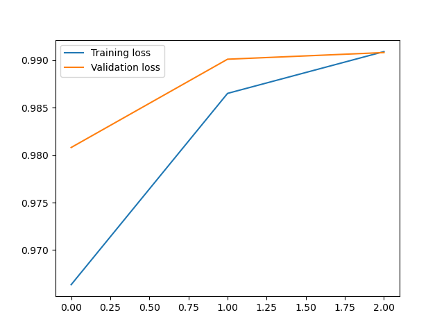
plt.plot(loss1, label='Training loss')
plt.plot(loss2, label='Validation loss')
plt.legend()
输出:
第0次训练:训练准确率:0.9646166666666718,测试准确率:0.9868999999999996
第1次训练:训练准确率:0.9865833333333389,测试准确率:0.9908999999999998
第2次训练:训练准确率:0.9917000000000039,测试准确率:0.9879999999999994
<matplotlib.legend.Legend at 0x21f03092fd0>