【pytorch】改造resnet為全卷積神經網路以適應不同大小的輸入
- 2020 年 4 月 1 日
- 筆記
為什麼resnet的輸入是一定的?
因為resnet最後有一個全連接層。正是因為這個全連接層導致了輸入的影像的大小必須是固定的。
輸入為固定的大小有什麼局限性?
原始的resnet在imagenet數據集上都會將影像縮放成224×224的大小,但這麼做會有一些局限性:
(1)當目標對象佔據影像中的位置很小時,對影像進行縮放將導致影像中的對象進一步縮小,影像可能不會正確被分類
(2)當影像不是正方形或對象不位於影像的中心處,縮放將導致影像變形
(3)如果使用滑動窗口法去尋找目標對象,這種操作是昂貴的
如何修改resnet使其適應不同大小的輸入?
(1)自定義一個自己網路類,但是需要繼承models.ResNet
(2)將自適應平均池化替換成普通的平均池化
(3)將全連接層替換成卷積層
相關程式碼:
import torch import torch.nn as nn from torchvision import models import torchvision.transforms as transforms from torch.hub import load_state_dict_from_url from PIL import Image import cv2 import numpy as np from matplotlib import pyplot as plt class FullyConvolutionalResnet18(models.ResNet): def __init__(self, num_classes=1000, pretrained=False, **kwargs): # Start with standard resnet18 defined here super().__init__(block = models.resnet.BasicBlock, layers = [2, 2, 2, 2], num_classes = num_classes, **kwargs) if pretrained: state_dict = load_state_dict_from_url( models.resnet.model_urls["resnet18"], progress=True) self.load_state_dict(state_dict) # Replace AdaptiveAvgPool2d with standard AvgPool2d self.avgpool = nn.AvgPool2d((7, 7)) # Convert the original fc layer to a convolutional layer. self.last_conv = torch.nn.Conv2d( in_channels = self.fc.in_features, out_channels = num_classes, kernel_size = 1) self.last_conv.weight.data.copy_( self.fc.weight.data.view ( *self.fc.weight.data.shape, 1, 1)) self.last_conv.bias.data.copy_ (self.fc.bias.data) # Reimplementing forward pass. def _forward_impl(self, x): # Standard forward for resnet18 x = self.conv1(x) x = self.bn1(x) x = self.relu(x) x = self.maxpool(x) x = self.layer1(x) x = self.layer2(x) x = self.layer3(x) x = self.layer4(x) x = self.avgpool(x) # Notice, there is no forward pass # through the original fully connected layer. # Instead, we forward pass through the last conv layer x = self.last_conv(x) return x
需要注意的是我們將全連接層的參數拷貝到自己定義的卷積層中去了。
看一下網路結構,主要是關注網路的最後:
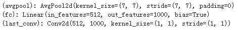
我們將self.avgpool替換成了AvgPool2d,而全連接層雖然還在網路中,但是在前向傳播時我們並沒有用到 。
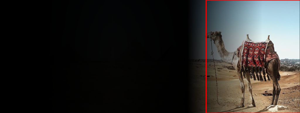
現在我們有這麼一張影像:

影像大小為:(387, 1024, 3)。而且目標對象駱駝是位於影像的右下角的。
我們就以這張圖片看一下是怎麼使用的。
with open('imagenet_classes.txt') as f: labels = [line.strip() for line in f.readlines()] # Read image original_image = cv2.imread('camel.jpg')# Convert original image to RGB format image = cv2.cvtColor(original_image, cv2.COLOR_BGR2RGB) # Transform input image # 1. Convert to Tensor # 2. Subtract mean # 3. Divide by standard deviation transform = transforms.Compose([ transforms.ToTensor(), #Convert image to tensor. transforms.Normalize( mean=[0.485, 0.456, 0.406], # Subtract mean std=[0.229, 0.224, 0.225] # Divide by standard deviation )]) image = transform(image) image = image.unsqueeze(0) # Load modified resnet18 model with pretrained ImageNet weights model = fcresnet18.FullyConvolutionalResnet18(pretrained=True).eval() print(model) with torch.no_grad(): # Perform inference. # Instead of a 1x1000 vector, we will get a # 1x1000xnxm output ( i.e. a probabibility map # of size n x m for each 1000 class, # where n and m depend on the size of the image.) preds = model(image) preds = torch.softmax(preds, dim=1) print('Response map shape : ', preds.shape) # Find the class with the maximum score in the n x m output map pred, class_idx = torch.max(preds, dim=1) print(class_idx) row_max, row_idx = torch.max(pred, dim=1) col_max, col_idx = torch.max(row_max, dim=1) predicted_class = class_idx[0, row_idx[0, col_idx], col_idx] # Print top predicted class print('Predicted Class : ', labels[predicted_class], predicted_class)
說明:imagenet_classes.txt中是標籤資訊。在數據增強時,並沒有將影像重新調整大小。用opencv讀取的圖片的格式為BGR,我們需要將其轉換為pytorch的格式:RGB。同時需要使用unsqueeze(0)增加一個維度,變成[batchsize,channel,height,width]。看一下avgpool和last_conv的輸出的維度:
我們使用torchsummary庫來進行每一層輸出的查看:
device = torch.device("cuda" if torch.cuda.is_available() else "cpu") model.to(device) from torchsummary import summary summary(model, (3, 387, 1024))
結果:
---------------------------------------------------------------- Layer (type) Output Shape Param # ================================================================ Conv2d-1 [-1, 64, 194, 512] 9,408 BatchNorm2d-2 [-1, 64, 194, 512] 128 ReLU-3 [-1, 64, 194, 512] 0 MaxPool2d-4 [-1, 64, 97, 256] 0 Conv2d-5 [-1, 64, 97, 256] 36,864 BatchNorm2d-6 [-1, 64, 97, 256] 128 ReLU-7 [-1, 64, 97, 256] 0 Conv2d-8 [-1, 64, 97, 256] 36,864 BatchNorm2d-9 [-1, 64, 97, 256] 128 ReLU-10 [-1, 64, 97, 256] 0 BasicBlock-11 [-1, 64, 97, 256] 0 Conv2d-12 [-1, 64, 97, 256] 36,864 BatchNorm2d-13 [-1, 64, 97, 256] 128 ReLU-14 [-1, 64, 97, 256] 0 Conv2d-15 [-1, 64, 97, 256] 36,864 BatchNorm2d-16 [-1, 64, 97, 256] 128 ReLU-17 [-1, 64, 97, 256] 0 BasicBlock-18 [-1, 64, 97, 256] 0 Conv2d-19 [-1, 128, 49, 128] 73,728 BatchNorm2d-20 [-1, 128, 49, 128] 256 ReLU-21 [-1, 128, 49, 128] 0 Conv2d-22 [-1, 128, 49, 128] 147,456 BatchNorm2d-23 [-1, 128, 49, 128] 256 Conv2d-24 [-1, 128, 49, 128] 8,192 BatchNorm2d-25 [-1, 128, 49, 128] 256 ReLU-26 [-1, 128, 49, 128] 0 BasicBlock-27 [-1, 128, 49, 128] 0 Conv2d-28 [-1, 128, 49, 128] 147,456 BatchNorm2d-29 [-1, 128, 49, 128] 256 ReLU-30 [-1, 128, 49, 128] 0 Conv2d-31 [-1, 128, 49, 128] 147,456 BatchNorm2d-32 [-1, 128, 49, 128] 256 ReLU-33 [-1, 128, 49, 128] 0 BasicBlock-34 [-1, 128, 49, 128] 0 Conv2d-35 [-1, 256, 25, 64] 294,912 BatchNorm2d-36 [-1, 256, 25, 64] 512 ReLU-37 [-1, 256, 25, 64] 0 Conv2d-38 [-1, 256, 25, 64] 589,824 BatchNorm2d-39 [-1, 256, 25, 64] 512 Conv2d-40 [-1, 256, 25, 64] 32,768 BatchNorm2d-41 [-1, 256, 25, 64] 512 ReLU-42 [-1, 256, 25, 64] 0 BasicBlock-43 [-1, 256, 25, 64] 0 Conv2d-44 [-1, 256, 25, 64] 589,824 BatchNorm2d-45 [-1, 256, 25, 64] 512 ReLU-46 [-1, 256, 25, 64] 0 Conv2d-47 [-1, 256, 25, 64] 589,824 BatchNorm2d-48 [-1, 256, 25, 64] 512 ReLU-49 [-1, 256, 25, 64] 0 BasicBlock-50 [-1, 256, 25, 64] 0 Conv2d-51 [-1, 512, 13, 32] 1,179,648 BatchNorm2d-52 [-1, 512, 13, 32] 1,024 ReLU-53 [-1, 512, 13, 32] 0 Conv2d-54 [-1, 512, 13, 32] 2,359,296 BatchNorm2d-55 [-1, 512, 13, 32] 1,024 Conv2d-56 [-1, 512, 13, 32] 131,072 BatchNorm2d-57 [-1, 512, 13, 32] 1,024 ReLU-58 [-1, 512, 13, 32] 0 BasicBlock-59 [-1, 512, 13, 32] 0 Conv2d-60 [-1, 512, 13, 32] 2,359,296 BatchNorm2d-61 [-1, 512, 13, 32] 1,024 ReLU-62 [-1, 512, 13, 32] 0 Conv2d-63 [-1, 512, 13, 32] 2,359,296 BatchNorm2d-64 [-1, 512, 13, 32] 1,024 ReLU-65 [-1, 512, 13, 32] 0 BasicBlock-66 [-1, 512, 13, 32] 0 AvgPool2d-67 [-1, 512, 1, 4] 0 Conv2d-68 [-1, 1000, 1, 4] 513,000 ================================================================ Total params: 11,689,512 Trainable params: 11,689,512 Non-trainable params: 0 ---------------------------------------------------------------- Input size (MB): 4.54 Forward/backward pass size (MB): 501.42 Params size (MB): 44.59 Estimated Total Size (MB): 550.55 ----------------------------------------------------------------
最後是看一下預測的結果:
Response map shape : torch.Size([1, 1000, 1, 4]) tensor([[[978, 980, 970, 354]]]) Predicted Class : Arabian camel, dromedary, Camelus dromedarius tensor([354])
與imagenet_classes.txt中對應(索引下標是從0開始的)

可視化關注點:
from google.colab.patches import cv2_imshow
# Find the n x m score map for the predicted class  score_map = preds[0, predicted_class, :, :].cpu().numpy()  score_map = score_map[0]    # Resize score map to the original image size  score_map = cv2.resize(score_map, (original_image.shape[1], original_image.shape[0]))    # Binarize score map  _, score_map_for_contours = cv2.threshold(score_map, 0.25, 1, type=cv2.THRESH_BINARY)  score_map_for_contours = score_map_for_contours.astype(np.uint8).copy()    # Find the countour of the binary blob  contours, _ = cv2.findContours(score_map_for_contours, mode=cv2.RETR_EXTERNAL, method=cv2.CHAIN_APPROX_SIMPLE)    # Find bounding box around the object.   rect = cv2.boundingRect(contours[0])  # Apply score map as a mask to original image  score_map = score_map - np.min(score_map[:])  score_map = score_map / np.max(score_map[:])  score_map = cv2.cvtColor(score_map, cv2.COLOR_GRAY2BGR)  masked_image = (original_image * score_map).astype(np.uint8)    # Display bounding box  cv2.rectangle(masked_image, rect[:2], (rect[0] + rect[2], rect[1] + rect[3]), (0, 0, 255), 2)    # Display images  #cv2.imshow("Original Image", original_image)  #cv2.imshow("activations_and_bbox", masked_image)  cv2_imshow(original_image)  cv2_imshow(masked_image)  cv2.waitKey(0)
在Googlecolab中ipynb要使用:from google.colab.patches import cv2_imshow
參考:https://www.learnopencv.com/cnn-receptive-field-computation-using-backprop/?ck_subscriber_id=503149816