3.Scikit-Learn實現完整的機器學習項目

• 2020 年 3 月 30 日
• 筆記

1       完整的機器學習項目

完成項目的步驟：

(1)    項目概述

(2)    獲取數據

(3)    發現並可視化數據，發現規律。

(4)    為機器學習演算法準備數據。

(5)    選擇模型，進行訓練。

(6)    微調模型。

(7)    給出解決方案。

(8)    部署、監控、維護系統。

1.1  使用真實數據

學習機器學習時，最好使用真實數據，而不是人工數據集。幸運的是，有上千個開源數據集 可以進行選擇，涵蓋多個領域。以下是一些可以查找的數據的地方：

流行的開源數據倉庫： UC  Irvine    Machine       Learning       Repository Kaggle     datasets Amazon’s  AWS      datasets 准入口（提供開源數據列表） http://dataportals.org/ http://opendatamonitor.eu/ http://quandl.com/ 其它列出流行開源數據倉庫的網頁： Wikipedia’s      list  of    Machine       Learning      datasets Quora.com   question Datasets subreddit

1.2  項目目標

你的第一個任務是利用加州普查數據，建立一個加州房價模型。然後根據其它指標，預測任何街區的的房價中位數。採用有監督的學習，這是一個多變數（街區人口，收入中位數）回歸任務。因為不需要對數據變動做出快速適應，所以採用批量學習（離線學習）。

1.3  選擇性能目標

選擇性能指標：預測值和實際值之間的差距作為系統預測誤差，通常用均方根誤差（m個實際值與預測值之差的平方，除以m的平均值，再開根號，得到均方根誤差），平均絕對偏差（實際值與預測值之差的絕對值的平均值）。K階閔氏範數（向量模的k次方之後，在開k次方根），切比雪夫範數（向量中最大的）。

1.4  核實假設

確定最終的目標是獲得準確的房屋價格，做投資評估，而不是給房屋價格進行分類高中低。不同的需求採用不同的分析方法和模型。

1.5  獲取程式碼和數據

（1）   獲取程式碼和數據

從https://github.com/ageron/handson-ml下載程式碼和數據，複製到路徑D:Projectpythonhandson-ml-master。

（2）   在window上安裝python和git用於模擬linux開發環境，設置環境變數

$ export HOME=”/d/project/python/handson-ml-master”

$ export ML_PATH=”$HOME/ml”

$ mkdir -p $ML_PATH

（3）   安裝庫模組和依賴，採用中國豆瓣的鏡像，國外的容易失敗。pip是python自帶的包管理器，可以通過命令下載模組和依賴。這樣下載

pip3 install –upgrade matplotlib jupyter numpy pandas scipy scikit-learn -i http://pypi.douban.com/simple/ –trusted-host pypi.douban.com

pip3安裝默認路徑是python的安裝目錄下的的依賴庫路徑D:PythonPython37Libsite-packages。項目是無法載入這個路徑的庫的，所以需要用–target指定項目庫路徑

pip3 install –upgrade numpy -i http://pypi.douban.com/simple/ –trusted-host pypi.douban.com –target=D:Projectpythonhandson-ml-mastervenvLibsite-packages

也可以在pycharm上設置下載地址進行下載。具體見部落格

https://www.cnblogs.com/bclshuai/p/12488341.html

jupyter nbconvert –to script 02_end_to_end_machine_learning_project.ipynb

啟動notebook的方法

有兩種，原理都相同，啟動jupyter的服務，進入目錄，讀取文件，運行文件。

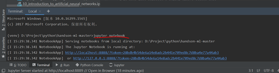
（1）在cmd命令行輸入jupyter notebook，會啟動Jupyter   伺服器，運行在終端上，監聽8888埠。你可以用瀏覽器打 開       http://localhost:8888/ 。然後可以咋瀏覽器中點擊new創建新的ipynb文件，進行編寫程式碼和網頁上測試運行。

（2）在pycharm的terminal窗口輸入jupyter notebook，也會啟動服務，一台電腦只能啟動一個服務，所以要關閉之前的cmd窗口。

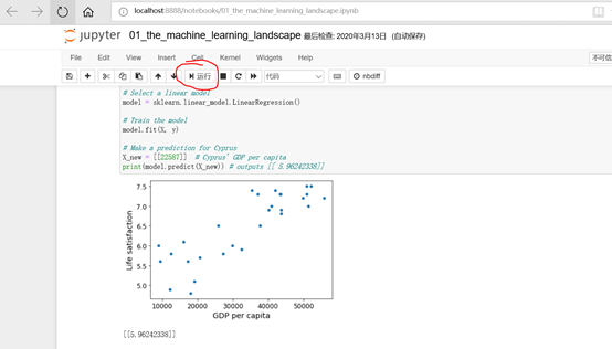
打開工程目錄

打開文件件01_the_machine_learning_landscape.ipynb，然後點擊運行按鈕，單步執行程式碼，會獲取數據畫出圖形。

1.5.1         下載數據

一般是要連接資料庫獲取數據，本文直接從github下載一個數據壓縮包，裡面是CSV資料庫文件。

（1）下載數據文件

import   os

import   tarfile from   six.moves     #壓縮文件處理

import   urllib # url下載操作

DOWNLOAD_ROOT      =       “https://raw.githubusercontent.com/ageron/handson-ml/master/” HOUSING_PATH      =     “datasets/housing” HOUSING_URL     =       DOWNLOAD_ROOT      +     HOUSING_PATH      +       “/housing.tgz”

def fetch_housing_data(housing_url=HOUSING_URL,housing_path=HOUSING_PATH):                           

if     not  os.path.isdir(housing_path):                                                            os.makedirs(housing_path)#如果不存在則創建數據目錄                          

tgz_path =     os.path.join(housing_path,      “housing.tgz”)#產生tgz文件路徑     urllib.request.urlretrieve(housing_url,  tgz_path)#下載壓縮文件                          

housing_tgz =     tarfile.open(tgz_path)#打開壓縮文件                       housing_tgz.extractall(path=housing_path)#解壓壓縮文件                       

housing_tgz.close()

（2）讀取數據

import pandas as pd

def load_housing_data(housing_path=HOUSING_PATH):
    csv_path = os.path.join(housing_path, “housing.csv”)
    return pd.read_csv(csv_path)

#%%

housing = load_housing_data()
housing.head()

（3）查看數據

#%%查看欄位定義屬性

housing.info()

#%%查看欄位ocean_proximity有那些值，每個值的統計分布

housing[“ocean_proximity”].value_counts()

#%%查看數據表中每個欄位的平均值，最大最小值，分布區間等

housing.describe()

#%%matplotlib  inline
#指定matplotlib使用jupyter的後端渲染圖片
%matplotlib inline
import matplotlib.pyplot as plt
#畫出每個屬性的柱狀圖
housing.hist(bins=50, figsize=(20,15))
save_fig(“attribute_histogram_plots”)
plt.show()

1.6  創建測試集

選用機器模型不能按照測試集的數據歸類選擇模型，否則容易測試正常，實際應用很糟。測試集需要保持固定性，不同次訓練測試，測試集的內容不變，需要採用固定的隨機因子進行取樣。

（1）   隨機取樣，每次獲取到的測試都不一樣。

#隨機取樣，用於說明
  def split_train_test(data, test_ratio):
      shuffled_indices = np.random.permutation(len(data))
      test_set_size = int(len(data) * test_ratio)
      test_indices = shuffled_indices[:test_set_size]
      train_indices = shuffled_indices[test_set_size:]
      return data.iloc[train_indices], data.iloc[test_indices]
  
  #%%隨機取樣
  
  train_set, test_set = split_train_test(housing, 0.2)
  print(len(train_set), "train +", len(test_set), "test")

（2）   固定的隨機種子取樣。隨機取樣每次採集的測試都不同，可以第一次採集後保存，或者採用固定的隨機種子取樣。

#%%
  #不同次訓練測試，測試集的內容不變，需要採用固定的隨機因子進行取樣。
  # to make this notebook's output identical at every run
  np.random.seed(42)

（3）   數據id哈希值計算取樣。如果數據集更新，或者進行了順序調整，則又會產生不同的測試集。可以根據每條記錄的id值計算出哈希值，最後一個位元組小於51（256的20%）的作為測試集數據，這樣無論數據集怎麼調整變化，只要每條記錄的id值不變，最後都可以獲取到相同的數據集。id可以有很多種。

#%%通過id計算來取樣
  
  from zlib import crc32
  
  def test_set_check(identifier, test_ratio):
      return crc32(np.int64(identifier)) & 0xffffffff < test_ratio * 2**32
  
  def split_train_test_by_id(data, test_ratio, id_column):
      ids = data[id_column]
      in_test_set = ids.apply(lambda id_: test_set_check(id_, test_ratio))
      return data.loc[~in_test_set], data.loc[in_test_set]
  
  #%% md
  
  The implementation of `test_set_check()` above works fine in both Python 2 and Python 3. In earlier releases, the following implementation was proposed, which supported any hash function, but was much slower and did not support Python 2:
  
  #%%採用id的hash值來取樣
  
  import hashlib
  
  def test_set_check(identifier, test_ratio, hash=hashlib.md5):
      return hash(np.int64(identifier)).digest()[-1] < 256 * test_ratio
  
  #%% md
  
  If you want an implementation that supports any hash function and is compatible with both Python 2 and Python 3, here is one:
  
  #%%
  
  def test_set_check(identifier, test_ratio, hash=hashlib.md5):
      return bytearray(hash(np.int64(identifier)).digest())[-1] < 256 * test_ratio
  
  #%%
  
  housing_with_id = housing.reset_index()   # adds an `index` column
  train_set, test_set = split_train_test_by_id(housing_with_id, 0.2, "index")

（4）   經緯度計算值取樣。如果沒有id值，可以根據欄位經緯度去計算判斷。

housing_with_id["id"] = housing["longitude"] * 1000 + housing["latitude"]
  train_set, test_set = split_train_test_by_id(housing_with_id, 0.2, "id")

（5）   Scikit-Learn自帶的取樣函數train_test_split。它有一個  random_state      參數，可以設定前面講過的隨機生成器種子；第二，你可 以將種子傳遞給多個行數相同的數據集，可以在相同的索引上分割數據集

#%%使用sklearn的train_test_split函數進行取樣分類
  
  from sklearn.model_selection import train_test_split
  
  train_set, test_set = train_test_split(housing, test_size=0.2, random_state=42)
  
  #%%

（6）   分層取樣。先把人按照不同的收入區間進行分類，再根據不同區間內的人數比例進行取樣。男女比例是3:1，則在男生裡面選擇75%的人，女生裡面選擇25%的人。

housing[“income_cat”] = np.ceil(housing[“median_income”] / 1.5)
# Label those above 5 as 5
housing[“income_cat”].where(housing[“income_cat”] < 5, 5.0, inplace=True)
“`

#%%按照收入進行分類，每個收入區間有多少人

housing[“income_cat”] = pd.cut(housing[“median_income”],
                               bins=[0., 1.5, 3.0, 4.5, 6., np.inf],
                               labels=[1, 2, 3, 4, 5])

#%%

housing[“income_cat”].value_counts()

#%%

housing[“income_cat”].hist()

#%%根據每個區間人數按照比例進行分層取樣。

from sklearn.model_selection import StratifiedShuffleSplit

split = StratifiedShuffleSplit(n_splits=1, test_size=0.2, random_state=42)
for train_index, test_index in split.split(housing, housing[“income_cat”]):
    strat_train_set = housing.loc[train_index]
    strat_test_set = housing.loc[test_index]

#%%

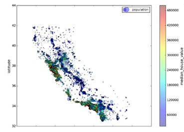
1.7  經緯度數據可視化

畫出經緯度影像，查看規律。

housing.plot(kind=”scatter”,   x=”longitude”,    y=”latitude”, alpha=0.4,                        s=housing[“population”]/100, label=”population”,                        c=”median_house_value”,      cmap=plt.get_cmap(“jet”),       colorbar=True, ) plt.legend()

1.8  查找關聯性

因為數據集並不是非常大，你可以很容易地使用       corr()     方法計算出每對屬性間的標準相關係 數（standard correlation   coefficient，也稱作皮爾遜相關係數）：

corr_matrix =     housing.corr()

（1）查看各屬性與median_house_value的相關性：

>>> corr_matrix[“median_house_value”].sort_values(ascending=False)

median_house_value                      1.000000

median_income                                                          0.687170

total_rooms                                                                        0.135231 housing_median_age                      0.114220

households                                                                                0.064702 total_bedrooms                                                    0.047865

population                                                                          -0.026699

longitude                                                                                   -0.047279

latitude                                                                                      -0.142826

（2）用Pandas的scatter_matrix    函數畫出主要屬性的影像

from      pandas.tools.plotting import   scatter_matrix

attributes      =     [“median_house_value”,  “median_income”,       “total_rooms”,                                                                                               “housing_median_age”] scatter_matrix(housing[attributes],       figsize=(12,  8))

1.9  組合屬性關聯性測試

創建一些關聯屬性，例如每個房子的房間數，每個房間的床數，每個房子的人口數。

housing[“rooms_per_household”]  =       housing[“total_rooms”]/housing[“households”] housing[“bedrooms_per_room”]    =       housing[“total_bedrooms”]/housing[“total_rooms”] housing[“population_per_household”]=housing[“population”]/housing[“households”]

重新計算關聯關係，得到新的關聯性排列，rooms_per_household變成第三關聯參數，即每個房子的房間數

>>> corr_matrix  =     housing.corr()

>>> corr_matrix[“median_house_value”].sort_values(ascending=False) median_house_value                                                                1.000000 median_income                                                                        0.687170

rooms_per_household                                                             0.199343

total_rooms                                                                               0.135231 housing_median_age                                                                0.114220

households                                                                                0.064702 total_bedrooms                                                                         0.047865 population_per_household                                                       -0.021984

population                                                                                 0.026699

longitude                                                                                   -0.047279

latitude                                                                                      -0.142826

bedrooms_per_room                                                                 -0.260070

Name:   median_house_value, dtype:    float64

1.10         數據訓練準備

1.10.1      數據轉換函數

創建一些數據轉換函數，方便地進行重複數據轉換，可以用於其他項目。

1.10.2      數據清洗缺失值記錄

去除處理

數據中有些屬性沒有，會對訓練造成影響，處理方法有

（1）   去掉缺失的記錄

housing.dropna(subset=[“total_bedrooms”])                           #     選項1

（2）   去掉整個屬性列

housing.drop(“total_bedrooms”,    axis=1)                                            #       選項2

（3）   用0，平均值，中位數去填充

median  =     housing[“total_bedrooms”].median() housing[“total_bedrooms”].fillna(median)                              #     選項3

Scikit-Learn      提供了一個方便的類來處理缺失值：Imputer

（1）   新建一個Imputer對象

（2）   imputer.fit（）計算中位數

（3）   imputer.transform（）預設值替換為中位數

#%%創建缺失值處理對象
  
  try:
      from sklearn.impute import SimpleImputer # Scikit-Learn 0.20+
  except ImportError:
      from sklearn.preprocessing import Imputer as SimpleImputer
  
  imputer = SimpleImputer(strategy="median")
  
  #%% md
  
  Remove the text attribute because median can only be calculated on numerical attributes:
  
  #%%只有數值才能計算中位數，去除文本變數ocean_proximity
  
  housing_num = housing.drop('ocean_proximity', axis=1)
  # alternatively: housing_num = housing.select_dtypes(include=[np.number])
  
  #%%擬合運算
  
  imputer.fit(housing_num)
  
  #%%imputer 計算出了每個屬性的中位數，並將結果保存在了實例變數  statistics_    中。
  
  imputer.statistics_
  
  #%% md
  
  Check that this is the same as manually computing the median of each attribute:
  
  #%%
  
  housing_num.median().values
  
  #%% md
  
  Transform the training set:
  
  #%%處理數據，預設值替換為中位數
  
  X = imputer.transform(housing_num)

1.11         Scikit-Learn  的  API     設計

介面一致性

（1）   估計器（timator）。imputer就是一個估計器，基於數據集對一些參數進行估計的對象為估計器。

（2）   轉換器transformer。對數據集進行轉化換。通過transferm（）方法

（3）   預測器（predictor）。根據給出的數據集做出預測。有一個redict（）方法。

1.12         處理文本和類別屬性

需要將文本屬性轉換為數字屬性，方便計算。

Scikit-Learn 為這個任務提供了一個轉換器    LabelEncoder     ：

>>> from      sklearn.preprocessing import   LabelEncoder

>>> encoder =     LabelEncoder()

>>> housing_cat  =     housing[“ocean_proximity”] #獲取屬性列

>>> housing_cat_encoded =     encoder.fit_transform(housing_cat) #轉換為數字

>>> housing_cat_encoded#輸出展示

array([1, 1,    4,    …,   1,    0,    3])

1.12.1      文本轉換方法

（1）   單文本轉換。

from      sklearn.preprocessing import   LabelEncoder >>>     encoder       =LabelEncoder()

housing_cat_encoded =     encoder.fit_transform(housing_cat)

（2）   多文本列轉換。

housing_cat_encoded =     housing_cat.factorize()

（3）   獨熱編碼OneHotEncoder

列中有很多個值：’1H    OCEAN’       ‘INLAND’     ‘ISLAND’     ‘NEAR       BAY’     ‘NEAR   OCEAN’，把列轉換為一個矩陣，只有值與對應位置的值相等才為1，其他都等於0。例如INLAND對的行為[0,1,0,0,0]

>>> from      sklearn.preprocessing import   OneHotEncoder >>> encoder       =     OneHotEncoder() #新建編碼對象

>>> housing_cat_1hot      =       encoder.fit_transform(housing_cat_encoded.reshape(-1,1)) #進行轉換

>>> housing_cat_1hot#返回一個矩陣

 <16513×5   sparse    matrix   of    type ‘<class   ‘numpy.float64′>’                     with       16513    stored    elements       in    Compressed Sparse       Row       format>

housing_cat_1hot.toarray() #轉換為數組n行5列的二維數組。

（4）LabelBinarizer實現一步執行這兩個轉換（從文本分類到整數分類，再從整 數分類到獨熱向量）：

>>> from      sklearn.preprocessing import   LabelBinarizer >>>   encoder       =     LabelBinarizer()

>>> housing_cat_1hot=encoder.fit_transform(housing_cat)

輸出結果和（3）中的相同。

array([[0,      1,    0,    0,    0],                                            

[0,   1,    0,    0,    0],                                            

[0,   0,    0,    0,    1],                                            

…,                                            

[0,   1,    0,    0,    0],                                            

[1,   0,    0,    0,    0],                                            

[0,   0,    0,    1,    0]])

（5）CategoricalEncoder實現多文本列轉換

#from    sklearn.preprocessing import   CategoricalEncoder   #     in       future    versions of    Sci kit-Learn

cat_encoder =     CategoricalEncoder()

housing_cat_reshaped      =     housing_cat.values.reshape(-1,      1)

housing_cat_1hot      =       cat_encoder.fit_transform(housing_cat_reshaped) housing_cat_1hot

1.13         特徵縮放

數據的取值範圍不同，例如總房間數分布範圍是6到39320，而收入中位數只分布在0到15，機器學習演算法的性能會不好。所以需要將所有屬性縮放為相同的度量。有兩種常見的方法可以讓所有的屬性有相同的量度：

線性函數歸一化（Min-Max scaling）：線性函數歸一化（許多人稱其為歸一化（normalization））很簡單：值被轉變、重新縮放， 直到範圍變成  0     到   1。我們通過減去最小值，然後再除以最大值與最小值的差值，來進行歸 一化。Scikit-Learn       提供了一個轉換器       MinMaxScaler    來實現這個功能

標準化（standardization）：首先減去平均值（所以標準化值的平均值總是      0），然後除以方差，使得到 的分布具有單位方差。Scikit-Learn     提供了一個轉換 器 StandardScaler    來進行標準化。

1.14         轉換流水線

1.14.1      多個轉換合成一個流水線

Scikit-Learn 提供 了類   Pipeline，將多個轉換合成一個流水線，按照順序執行。

from      sklearn.pipeline  import   Pipeline from       sklearn.preprocessing import   StandardScaler

num_pipeline      =     Pipeline([                                                     (‘imputer’,     Imputer(strategy=”median”)),                                                  (‘attribs_adder’,   CombinedAttributesAdder()),                                                  (‘std_scaler’, StandardScaler()),                                                       ])

housing_num_tr  =     num_pipeline.fit_transform(housing_num)

1.14.2      FeatureUnion將多個流水線轉換為同一個流水線

from      sklearn.pipeline  import   FeatureUnion

num_attribs  =     list(housing_num) cat_attribs  =     [“ocean_proximity”]

#流水線1

num_pipeline      =     Pipeline([(‘selector’,       DataFrameSelector(num_attribs)),                                                  (‘imputer’,     Imputer(strategy=”median”)),                                                  (‘attribs_adder’,   CombinedAttributesAdder()),                                                  (‘std_scaler’, StandardScaler()),                           ])

#流水線2

cat_pipeline =     Pipeline([(‘selector’,   DataFrameSelector(cat_attribs)),                                                   (‘label_binarizer’, LabelBinarizer()),])

#合併流水線

full_pipeline =     FeatureUnion(transformer_list=[                                                   (“num_pipeline”, num_pipeline),                                                    (“cat_pipeline”,  cat_pipeline),                           ])

#運行流水線

housing_prepared      =     full_pipeline.fit_transform(housing)

1.15         選擇並訓練模型

1.15.1      採用線性回歸模型去擬合

（1）模型訓練

from      sklearn.linear_model import   LinearRegression

housing_labels    =     strat_train_set[“median_house_value”].copy()#訓練集的房屋中位數原始值

lin_reg   =     LinearRegression()

lin_reg.fit(housing_prepared,  housing_labels)

（2）取前五個值驗證預測值

>>> some_data    =     housing.iloc[:5]#取前5個訓練值

>>>some_labels =     housing_labels.iloc[:5]#取前五個原始值

>>>some_data_prepared  =     full_pipeline.transform(some_data) #轉換

>>> print(“Predictions:t”, lin_reg.predict(some_data_prepared)) #模型預測

Predictions:  [      303104.               44800.          308928.        294208.        368704.]

>>> print(“Labels:tt”,     list(some_labels))#目標原始值展示

Labels:  [359400.0,    69700.0,       302100.0,     301300.0,     351900.0]

（3）採用均方差驗證預測值和原始值之間的差異

>>> from      sklearn.metrics   import   mean_squared_error

>>> housing_predictions  =     lin_reg.predict(housing_prepared) #獲取預測值

>>> lin_mse =     mean_squared_error(housing_labels,       housing_predictions) #求均方差

>>> lin_rmse       =     np.sqrt(lin_mse)

 >>>lin_rmse

68628.413493824875

均方差太大，欠擬合。

1.15.2      決策樹回歸模型訓練

（1）模型訓練

from      sklearn.tree  import   DecisionTreeRegressor

tree_reg =     DecisionTreeRegressor()

tree_reg.fit(housing_prepared, housing_labels)

（2）均方差驗證

>>> housing_predictions  =     tree_reg.predict(housing_prepared)

 >>>     tree_mse      =     mean_squared_error(housing_labels,       housing_predictions)

 >>>     tree_rmse     =     np.sqrt(tree_mse)

>>> tree_rmse 0.0

均方差為0，這裡用的是訓練集去驗證，過擬合，用測試集去測試更好。

1.15.3      使用交叉驗證做更佳的評估

K折交叉驗證（K-fold  cross-validation）上述的訓練方法並不是很好，一般是將訓練集分成K個子集，1個子集做測試集，其他K-1個子集做訓練集，做K次訓練和驗證。

（1）模型訓練

from      sklearn.model_selection   import   cross_val_score

 scores  =     cross_val_score(tree_reg, housing_prepared,       housing_labels,   scoring=”neg_mean_squared_error”,    cv=10)

rmse_scores =     np.sqrt(-scores)

（2）定義一個顯示評分的函數

def  display_scores(scores):

print(“Scores:”,      scores)               

print(“Mean:”, scores.mean()) …                           

print(“Standard      deviation:”,  scores.std())

（3）調用函數顯示評分

display_scores(tree_rmse_scores) Scores:   [      74678.4916885                 64766.2398337                 69632.86942005        69166.67693232                                                                71486.76507766        73321.65695983        71860.04741226        71086.32691692                                                                76934.2726093                 69060.93319262]

 Mean:  71199.4280043 Standard  deviation:     3202.70522793

（4）   線性模型的10折交叉驗證對比

lin_scores     =     cross_val_score(lin_reg,   housing_prepared,       housing_labels,

                                                                                                                                                                                                           scoring=”neg_mean_squared_error”,    cv=10)

>>> lin_rmse_scores  =     np.sqrt(-lin_scores)

 >>>     display_scores(lin_rmse_scores)

 Scores: [      70423.5893262                 65804.84913139        66620.84314068        72510.11362141                                                                66414.74423281        71958.89083606        67624.90198297              67825.36117664                                                                72512.36533141        68028.11688067]

Mean:    68972.377566 Standard    deviation:     2493.98819069

線性模型比決策樹模型的均值和方差更小。決策樹模型過擬合很嚴重，它的性能比線性回歸模型還差。

1.15.4      隨機森林模型

隨機森林是通過用特 征的隨機子集訓練許多決策樹。在其它多個模型之上建立模型稱為集成學習（Ensemble Learning）

>>> from      sklearn.ensemble import   RandomForestRegressor

>>> forest_reg     =     RandomForestRegressor()

>>> forest_reg.fit(housing_prepared,    housing_labels)

>>> forest_rmse 22542.396440343684

>>> display_scores(forest_rmse_scores) Scores: [      53789.2879722                 50256.19806622        52521.55342602        53237.44937943                                                                52428.82176158        55854.61222549        52158.02291609        50093.66125649                                                                53240.80406125       52761.50852822]

 Mean:  52634.1919593 Standard  deviation:     1576.20472269

1.16         模型微調

對模型的參數進行調整，優化模型，減少誤差。手動調整參數效率低而且不容易獲得較優的參數。可以採用下面幾種方法來獲取最優參數。

1.16.1      網格檢索GridSearchCV

將參數可能的取值放入一個參數數組中，每個參數有幾個值，如下面的參數網格，{‘n_estimators’: [3,   10,  30], ‘max_features’:    [2,   4,    6,       8]}有3*4=12種組合。{‘bootstrap’:    [False],  ‘n_estimators’:     [3,       10], ‘max_features’:    [2,   3,4]}+ 1*2*3=6種組合。一共有18組參數用來訓練數據集。每組參數再採用5折交叉驗證，則需要進行18*5=90論訓練。

from      sklearn.model_selection   import   GridSearchCV

param_grid =     [      {‘n_estimators’:   [3,   10,  30], ‘max_features’:    [2,       4,    6,    8]}, {‘bootstrap’: [False],  ‘n_estimators’:     [3,   10],       ‘max_features’:    [2,   3,    4]},        ]

forest_reg     =     RandomForestRegressor()

grid_search  =     GridSearchCV(forest_reg,     param_grid, cv=5,                                                                                                                                                                                           scoring=’neg_mean_squared_error’)

grid_search.fit(housing_prepared, housing_labels)

#查看最優參數

>>> grid_search.best_params_

{‘max_features’:  6,    ‘n_estimators’:     30}

#查看最佳估計器

>>> grid_search.best_estimator_

RandomForestRegressor(bootstrap=True,   criterion=’mse’,       max_depth=None,                                                                           max_features=6, max_leaf_nodes=None,    min_samples_leaf=1,                                                                       min_samples_split=2,       min_weight_fraction_leaf=0.0,                                                                            n_estimators=30, n_jobs=1,     oob_score=False,       random_state=None,                                                                       verbose=0,   warm_start=False)

#查看所有評分

>>> cvres      =     grid_search.cv_results_ … for  mean_score, params  in       zip(cvres[“mean_test_score”], cvres[“params”]): …                               print(np.sqrt(-mean_score),     params) …

 64912.0351358 {‘max_features’:  2,    ‘n_estimators’:     3}

55535.2786524   {‘max_features’:  2,    ‘n_estimators’:     10}

52940.2696165   {‘max_features’:  2,    ‘n_estimators’:     30}

60384.0908354   {‘max_features’:  4,    ‘n_estimators’:     3}

52709.9199934   {‘max_features’:  4,    ‘n_estimators’:     10}

50503.5985321   {‘max_features’:  4,    ‘n_estimators’:     30}

59058.1153485   {‘max_features’:  6,    ‘n_estimators’:     3}

52172.0292957   {‘max_features’:  6,    ‘n_estimators’:     10}

49958.9555932   {‘max_features’:       6,    ‘n_estimators’:  30} #最優參數

59122.260006     {‘max_features’:  8,    ‘n_estimators’:     3}

52441.5896087   {‘max_features’:  8,    ‘n_estimators’:     10}

50041.4899416   {‘max_features’:  8,    ‘n_estimators’:     30}

62371.1221202   {‘bootstrap’:  False,     ‘max_features’:    2,       ‘n_estimators’:     3} 54572.2557534     {‘bootstrap’:  False,       ‘max_features’:    2,    ‘n_estimators’:     10} 59634.0533132       {‘bootstrap’:  False,     ‘max_features’:    3,    ‘n_estimators’:     3} 52456.0883904   {‘bootstrap’:  False,     ‘max_features’:    3,       ‘n_estimators’:     10} 58825.665239     {‘bootstrap’:  False,       ‘max_features’:    4,    ‘n_estimators’:     3} 52012.9945396       {‘bootstrap’:  False,     ‘max_features’:    4,    ‘n_estimators’:     10}

1.16.2      隨機搜索RandomizedSearchCV

當超參數的搜索空間很大時，不適合用網格搜索，適合用RandomizedSearchCV，它不 是嘗試所有可能的組合，而是通過選擇每個超參數的一個隨機值的特定數量的隨機組合。通過設置搜索次數控制計算量。

1.17         用測試集評估系統

用網格檢索的最優模型計算預測值和實際值進行比較，計算出誤差和均方差。

final_model =     grid_search.best_estimator_

X_test    =     strat_test_set.drop(“median_house_value”, axis=1) #去除房價中位數的數據

y_test    =     strat_test_set[“median_house_value”].copy()#實際值

X_test_prepared =     full_pipeline.transform(X_test)#測試集進行同等轉換

final_predictions =     final_model.predict(X_test_prepared)#計算預測值

final_mse     =     mean_squared_error(y_test,    final_predictions) #誤差

final_rmse    =     np.sqrt(final_mse)                  

#     =>  evaluates      to    48,209.6

1.18         啟動、監控、維護系統

啟動系統用於實際應用， 編寫監控程式監測系統的系統，咋系統性能下降時給出報警。模型性能會下降，除非模型用新數據定期訓練。你還要評估系統輸入數據的品質，低品質的訊號（比如失靈的感測器發送隨機值， 或另一個團隊的輸出停滯），系統的表現會逐漸變差，但可能需要一段時間，系統的表現才 能下降到一定程度，觸發警報。

自己開發了一個股票智慧分析軟體，功能很強大，需要的點擊下面的鏈接獲取：

https://www.cnblogs.com/bclshuai/p/11380657.html