CTR學習筆記&程式碼實現1-深度學習的前奏LR->FFM
- 2020 年 3 月 16 日
- 筆記
CTR學習筆記系列的第一篇,總結在深度模型稱王之前經典LR,FM, FFM模型,這些經典模型後續也作為組件用於各個深度模型。模型分別用自定義Keras Layer和estimator來實現,哈哈一個是舊愛一個是新歡。特徵工程依賴feature_column實現,這裡做的比較簡單在後面的深度模型再好好搞。完整程式碼在這裡https://github.com/DSXiangLi/CTR
問題定義
CTR本質是一個二分類問題,$X in R^N $是用戶和廣告相關特徵, (Y in (0,1))是每個廣告是否被點擊,基礎模型就是一個簡單的Logistics Regression
[ P(Y=1) = frac{1}{1+ exp{(w_0 + sum_{i=1}^Nw_ix_i)}} ]
考慮在之後TF框架里logistics可以簡單用activation來表示,我們把核心的部分簡化為以下
[ y(x) = w_0 + sum_{i=1}^Nw_ix_i ]

LR模型
2010年之前主流的CTR模型通常是最簡單的logistics regression,模型可解釋性強,工程上部署簡單快捷。但最大的問題是依賴於大量的手工特徵工程。
剛接觸特徵工程的同學可能會好奇為什麼需要計算組合特徵?
最開始我只是簡單認為越細粒度的聚合特徵Bias越小。接觸了因果推理後,我覺得更適合用Simpson Paradox里的Confounder Bias來解釋,不同聚合特徵之間可能會相悖,例如各個年齡段的男性點擊率均低於女性,但整體上男性的點擊率高於女性。感興趣的可以看看這篇部落格因果推理的春天系列序 – 數據挖掘中的Confounding, Collidar, Mediation Bias
如果即想簡化特徵工程,又想加入特徵組合,肯定就會想到下面的暴力特徵組合方式。這個也被稱作POLY2模型
[ y(x) = w_0 + sum_{i=1}^N w_ix_i + sum_{i=1}^N sum_{j=i+1}^N w_{i,j} x_ix_j ]
但上述(w_{i,j})需要學習(frac{n(n-1)}{2})個參數,一方面複雜度高,另一方面對高維稀疏特徵會出現大量(w_{i,j})是0的情況,模型無法學到樣本中未曾出現的特徵組合pattern,模型泛化性差。
於是降低複雜度,自動選擇有效特徵組合,以及模型泛化這三點成為後續主要的改進的方向。
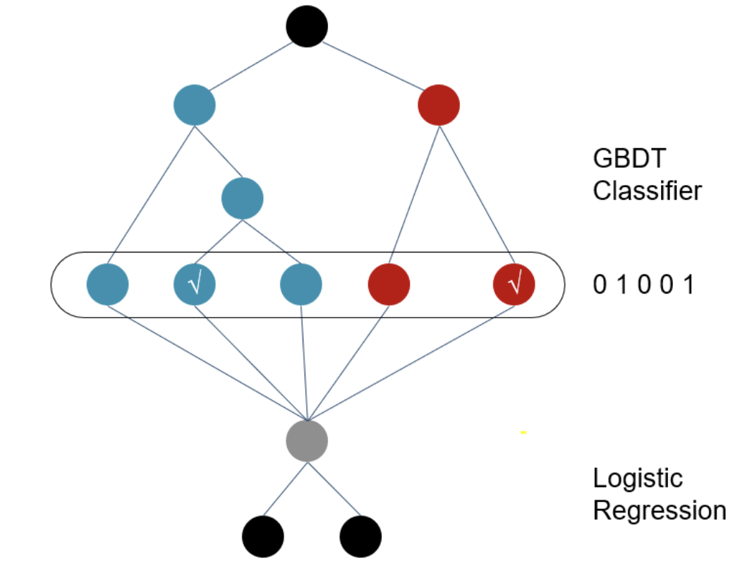
GBDT+LR模型
2014年Facebook提出在GBDT疊加LR的方法,敲開了特徵工程模型化的大門。GBDT輸出的不是預測概率,而是每一個樣本落在每一顆子樹哪個葉節點的一個0/1矩陣。在只保留和target相關的有效特徵組合的同時,避免了手工特徵組合需要的業務理解和人工成本。
相較特徵組合,我更喜歡把GBDT輸出的特徵向量,理解為根據target,對樣本進行了聚類/降維,輸出的是該樣本所屬的幾個特定人群組合,每一棵子樹都對應一種類型的人群組合。
但是!GBDT依舊存在泛化問題,因為所有葉節點的選擇都依賴於訓練樣本,並且GBDT在離散特徵上效果比較有限。同時也存在經過GBDT變換得到的特徵依舊是高維稀疏特徵的問題。
FM模型
2010年Rendall提出的因子分解機模型(FM)為降低計算複雜度,為增加模型泛化能力提供了思路
原理
FM模型將上述暴力特徵組合直接求解整個權重矩(w_ij in R^{N*N}),轉化為求解權重矩陣的隱向量(V in R^{N*k}),這一步會大大增加模型泛化能力,因為權重矩陣不再完全依賴於樣本中的特定特徵組合,而是可以通過特徵間的相關關係間接得到。 同時隱向量把模型需要學習的參數數量從(frac{n(n-1)}{2})降低到(nk)個
[ begin{align} y(x) & = w_0 + sum_{i=1}^Nw_i x_i + sum_{i=1}^N sum_{j=i+1}^N w_{i,j} x_ix_j\ &= w_0 + sum_{i=1}^Nw_i x_i + sum_{i=1}^N sum_{j=i+1}^N <v_i,v_j> x_ix_j\ end{align} ]
同時FM通過下面的trick,把擬合過程的計算複雜度從(O(n^2k))降低到線性複雜度(O(nk))
[ begin{align} &sum_{i=1}^N sum_{j=i+1}^N<v_i,v_j> x_ix_j \ = &frac{1}{2}( sum_{i=1}^N sum_{j=1}^N<v_i,v_j> x_ix_j – sum_{i=1}^N<v_i,v_i>x_ix_i)\ = &frac{1}{2}( sum_{i=1}^N sum_{j=1}^Nsum_{f=1}^K v_{if}v_{jf} x_ix_j – sum_{i=1}^Nsum_{f=1}^Kv_{if}^2x_i^2)\ = &frac{1}{2}sum_{f=1}^K( sum_{i=1}^N sum_{j=1}^N v_{if}v_{jf} x_ix_j – sum_{i=1}^Nv_{if}^2x_i^2)\ = &frac{1}{2}sum_{f=1}^K( (sum_{i=1}^N v_{ij}x_i)^2 – sum_{i=1}^Nv_{if}^2x_i^2)\ = &text{square_of_sum} -text{sum_of_square} end{align} ]
程式碼實現-自定義Keras Layer
class FM_Layer(Layer): """ Input: factor_dim: latent vector size input_shape: raw feature size activation output: FM layer output """ def __init__(self, factor_dim, activation = None, **kwargs): self.factor_dim = factor_dim self.activation = activations.get(activation) # if None return linear, else return function of identifier self.InputSepc = InputSpec(ndim=2) # Specifies input layer attribute. one Inspec for each input super(FM_Layer,self).__init__(**kwargs) def build(self, input_shape): """ input: tuple of input_shape output: w: linear weight v: latent vector b: linear Bias func: define all the necessary variable here """ assert len(input_shape) >=2 input_dim = int(input_shape[-1]) self.w = self.add_weight(name = 'w0', shape = (input_dim, 1), initializer = 'glorot_uniform', trainable = True) self.b = self.add_weight(name = 'bias', shape = (1, ), initializer = 'zeros', trainable = True) self.v = self.add_weight(name = 'hidden_vector', shape = (input_dim, self.factor_dim), initializer = 'glorot_uniform', trainable = True) super(FM_Layer, self).build(input_shape)# set self.built=True def call(self, x): """ input: x(previous layer output) output: core calculation of the FM layer func: core calculcation of layer goes here """ linear_term = K.dot(x, self.w) + self.b # Embedding之和,Embedding內積: (1, input_dim) * (input_dim, factor_dim) = (1, factor_dim) sum_square = K.pow(K.dot(x, self.v),2) square_sum = K.dot(K.pow(x, 2), K.pow(self.v, 2)) # (1, factor_dim) -> (1) quad_term = K.mean( (sum_square - square_sum), axis=1, keepdims = True) # output = self.activation((linear_term+quad_term)) return output def compute_output_shape(self, input_shape): # tf.keras回傳input_shape是tf.dimension而不是tuple, 所以要cast成int return (int(input_shape[0]), self.output_dim) FM和MF的關係
Factorizaton Machine 和Matrix Factorization聽起來就很像,MF也確實是FM的一個特例。MF是通過對矩陣進行因子分解得到隱向量,但因為只適用於矩陣所以特徵只能是二維,常見的是(user_id, item_id)組合。而同樣是得到隱向量,FM將矩陣展平把離散特徵都做one-hot,因此支援任意數量的輸入特徵。

FM和Embedding的關係
Embedding最常見於NLP中,把詞的高維稀疏特徵映射到低維矩陣embedding中,然後用交互函數,例如向量內積來表示詞與詞之間的相似度。而實際上FM計算的隱向量也是一種Embedding 的擬合方法,並且限制了只用向量內積作為交互函數。上述(X*V in R^{K})得到的就是Embedding向量本身。
FFM
2015年提出的FFM模型在FM的基礎上加入了Field的概念
原理
上述FM學到的權重矩陣V是每個特徵對應一個隱向量,兩特徵組合通過隱向量內積的形式來表達。FFM提出同一個特徵和不同Field的特徵組合應該有不同的隱向量,因此(V in R^{N*K})變成 (V in R^{N*F*K})其中F是特徵所屬Field的個數。以下數據中country,Data,Ad_type就是Field((F=3))

FM兩特徵交互的部分被改寫為以下,因此需要學習的參數數量從nk變為nf*k。並且在擬合過程中無法使用上述trick因此複雜度從FM的(O(nk))上升為(O(kn^2))。
[ begin{align} sum_{i=1}^N sum_{j=i+1}^N<v_i,v_j> x_ix_j to &sum_{i=1}^N sum_{j=i+1}^N<v_{i,f_j},v_{j,f_i}> x_ix_j end{align} ]
程式碼實現-自定義model_fn
def model_fn(features, labels, mode, params): """ Field_aware factorization machine for 2 classes classification """ feature_columns, field_dict = build_features() field_dim = len(np.unique(list(field_dict.values()))) input = tf.feature_column.input_layer(features, feature_columns) input_dim = input.get_shape().as_list()[-1] with tf.variable_scope('linear'): init = tf.random_normal( shape = (input_dim,2) ) w = tf.get_variable('w', dtype = tf.float32, initializer = init, validate_shape = False) b = tf.get_variable('b', shape = [2], dtype= tf.float32) linear_term = tf.add(tf.matmul(input,w), b) tf.summary.histogram( 'linear_term', linear_term ) with tf.variable_scope('field_aware_interaction'): init = tf.truncated_normal(shape = (input_dim, field_dim, params['factor_dim'])) v = tf.get_variable('v', dtype = tf.float32, initializer = init, validate_shape = False) interaction_term = tf.constant(0, dtype =tf.float32) # iterate over all the combination of features for i in range(input_dim): for j in range(i+1, input_dim): interaction_term += tf.multiply( tf.reduce_mean(tf.multiply(v[i, field_dict[j],: ], v[j, field_dict[i],:])) , tf.multiply(input[:,i], input[:,j]) ) interaction_term = tf.reshape(interaction_term, [-1,1]) tf.summary.histogram('interaction_term', interaction_term) with tf.variable_scope('output'): y = tf.math.add(interaction_term, linear_term) tf.summary.histogram( 'output', y ) if mode == tf.estimator.ModeKeys.PREDICT: predictions = { 'predict_class': tf.argmax(tf.nn.softmax(y), axis=1), 'prediction_prob': tf.nn.softmax(y) } return tf.estimator.EstimatorSpec(mode = tf.estimator.ModeKeys.PREDICT, predictions = predictions) cross_entropy = tf.reduce_mean(tf.nn.sparse_softmax_cross_entropy_with_logits( labels=labels, logits=y )) if mode == tf.estimator.ModeKeys.TRAIN: optimizer = tf.train.AdamOptimizer(learning_rate = params['learning_rate']) train_op = optimizer.minimize(cross_entropy, global_step = tf.train.get_global_step()) return tf.estimator.EstimatorSpec(mode, loss = cross_entropy, train_op = train_op) else: eval_metric_ops = { 'accuracy': tf.metrics.accuracy(labels = labels, predictions = tf.argmax(tf.nn.softmax(y), axis=1)), 'auc': tf.metrics.auc(labels = labels , predictions = tf.nn.softmax(y)[:,1]), 'pr': tf.metrics.auc(labels = labels, predictions = tf.nn.softmax(y)[:,1], curve = 'PR') } return tf.estimator.EstimatorSpec(mode, loss = cross_entropy, eval_metric_ops = eval_metric_ops) 參考資料
- S. Rendle, 「Factorization machines,」 in Proceedings of IEEE International Conference on Data Mining (ICDM), pp. 995–1000, 2010
- Yuchin Juan,Yong Zhuang,Wei-Sheng Chin,Field-aware Factorization Machines for CTR Prediction。
- 盤點前深度學習時代阿里、Google、Facebook的CTR預估模型
- 前深度學習時代CTR預估模型的演化之路:從LR到FFM
- 推薦系統召回四模型之:全能的FM模型
- 主流CTR預估模型的演化及對比
- 深入FFM原理與實踐