Pytorch之Spatial-Shift-Operation的5種實現策略
Pytorch之Spatial-Shift-Operation的5種實現策略
本文已授權極市平台, 並首發於極市平台公眾號. 未經允許不得二次轉載.
原始文檔(可能會進一步更新): //www.yuque.com/lart/ugkv9f/nnor5p
前言
之前看了一些使用空間偏移操作來替代區域卷積運算的論文:
- 粗看: //www.yuque.com/lart/architecture/conv#uKY5N
- (CVPR 2018) [Grouped Shift] Shift: A Zero FLOP, Zero Parameter Alternative to Spatial Convolutions:
- (ICCV 2019) 4-Connected Shift Residual Networks
- (NIPS 2018) [Active Shift] Constructing Fast Network through Deconstruction of Convolution
- (CVPR 2019) [Sparse Shift] All You Need Is a Few Shifts: Designing Efficient Convolutional Neural Networks for Image Classification
- 細看:
- Vision MLP之Hire-MLP Vision MLP via Hierarchical Rearrangement
- Hire-MLP: Vision MLP via Hierarchical Rearrangement://www.yuque.com/lart/papers/lbhadn
- Visoin MLP之CycleMLP A MLP-like Architecture for Dense Prediction
- CycleMLP: A MLP-like Architecture for Dense Prediction://www.yuque.com/lart/papers/om3xb6
- Vision MLP之S2-MLP V1&V2 Spatial-Shift MLP Architecture for Vision
- S2-MLP: Spatial-Shift MLP Architecture for Vision://www.yuque.com/lart/papers/dgdu2b
- S2-MLPv2: Improved Spatial-Shift MLP Architecture for Vision://www.yuque.com/lart/papers/dgdu2b
- Vision MLP之Hire-MLP Vision MLP via Hierarchical Rearrangement
看完這些論文後, 通過參考他們提供的核心程式碼(主要是後面那些MLP方法), 讓我對於實現空間偏移有了一些想法.
通過整合現有的知識, 我歸納總結了五種實現策略.
由於我個人使用pytorch, 所以這裡的展示也可能會用到pytorch自身提供的一些有用的函數.
問題描述
在提供實現之前, 我們應該先明確目的以便於後續的實現.
這些現有的工作都可以簡化為:
給定tensor \(X \in \mathbb{R}^{1 \times 8 \times 5 \times 5}\), 這裡遵循pytorch默認的數據格式, 即
B, C, H, W.通過變換操作\(\mathcal{T}: x \rightarrow \tilde{x}\), 將\(X\)轉換為\(\tilde{X}\).
這裡tensor \(\tilde{X} \in \mathbb{R}^{1 \times 8 \times 5 \times 5}\), 為了提供合理的對比, 這裡統一使用後面章節中基於”切片索引”策略的結果作為\(\tilde{X}\)的值.
import torch

xs = torch.meshgrid(torch.arange(5), torch.arange(5))
x = torch.stack(xs, dim=0)
x = x.unsqueeze(0).repeat(1, 4, 1, 1).float()
print(x)

'''
tensor([[[[0., 0., 0., 0., 0.],
          [1., 1., 1., 1., 1.],
          [2., 2., 2., 2., 2.],
          [3., 3., 3., 3., 3.],
          [4., 4., 4., 4., 4.]],

         [[0., 1., 2., 3., 4.],
          [0., 1., 2., 3., 4.],
          [0., 1., 2., 3., 4.],
          [0., 1., 2., 3., 4.],
          [0., 1., 2., 3., 4.]],

         [[0., 0., 0., 0., 0.],
          [1., 1., 1., 1., 1.],
          [2., 2., 2., 2., 2.],
          [3., 3., 3., 3., 3.],
          [4., 4., 4., 4., 4.]],

         [[0., 1., 2., 3., 4.],
          [0., 1., 2., 3., 4.],
          [0., 1., 2., 3., 4.],
          [0., 1., 2., 3., 4.],
          [0., 1., 2., 3., 4.]]]])
'''
方法1: 切片索引
這是最直接和簡單的策略了. 這也是S2-MLP系列中使用的策略.
我們將其作為其他所有策略的參考對象. 後續的實現中同樣會得到這個結果.
direct_shift = torch.clone(x)
direct_shift[:, 0:2, :, 1:] = torch.clone(direct_shift[:, 0:2, :, :4])
direct_shift[:, 2:4, :, :4] = torch.clone(direct_shift[:, 2:4, :, 1:])
direct_shift[:, 4:6, 1:, :] = torch.clone(direct_shift[:, 4:6, :4, :])
direct_shift[:, 6:8, :4, :] = torch.clone(direct_shift[:, 6:8, 1:, :])
print(direct_shift)

'''
tensor([[[[0., 0., 0., 0., 0.],
          [1., 1., 1., 1., 1.],
          [2., 2., 2., 2., 2.],
          [3., 3., 3., 3., 3.],
          [4., 4., 4., 4., 4.]],

         [[0., 0., 1., 2., 3.],
          [0., 0., 1., 2., 3.],
          [0., 0., 1., 2., 3.],
          [0., 0., 1., 2., 3.],
          [0., 0., 1., 2., 3.]],

         [[0., 0., 0., 0., 0.],
          [1., 1., 1., 1., 1.],
          [2., 2., 2., 2., 2.],
          [3., 3., 3., 3., 3.],
          [4., 4., 4., 4., 4.]],

         [[1., 2., 3., 4., 4.],
          [1., 2., 3., 4., 4.],
          [1., 2., 3., 4., 4.],
          [1., 2., 3., 4., 4.],
          [1., 2., 3., 4., 4.]],

         [[0., 0., 0., 0., 0.],
          [0., 0., 0., 0., 0.],
          [1., 1., 1., 1., 1.],
          [2., 2., 2., 2., 2.],
          [3., 3., 3., 3., 3.]],

         [[0., 1., 2., 3., 4.],
          [0., 1., 2., 3., 4.],
          [0., 1., 2., 3., 4.],
          [0., 1., 2., 3., 4.],
          [0., 1., 2., 3., 4.]],

         [[1., 1., 1., 1., 1.],
          [2., 2., 2., 2., 2.],
          [3., 3., 3., 3., 3.],
          [4., 4., 4., 4., 4.],
          [4., 4., 4., 4., 4.]],

         [[0., 1., 2., 3., 4.],
          [0., 1., 2., 3., 4.],
          [0., 1., 2., 3., 4.],
          [0., 1., 2., 3., 4.],
          [0., 1., 2., 3., 4.]]]])
'''
方法2: 特徵圖偏移—— torch.roll
pytorch提供了一個直接對特徵圖進行偏移的函數, 即 torch.roll . 這一操作在最近的transformer論文和mlp中有一些工作已經開始使用, 例如SwinTransformer和AS-MLP.
這裡展示下AS-MLP論文中提供的偽程式碼:
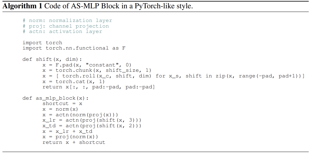
其主要作用就是將特徵圖沿著某個軸向進行偏移, 並支援同時沿著多個軸向偏移, 從而構造更多樣的偏移方向.
為了實現與前面相同的結果, 我們需要首先對輸入進行padding.
因為直接切片索引有個特點就是邊界值是會重複出現的, 而若是直接roll操作, 會導致所有的值整體移動.
所以為了實現類似的效果, 先對四周各padding一個網格的數據.
注意這裡選擇使用重複模式(replicate)以實現最終的邊界重複值的效果.
import torch.nn.functional as F

pad_x = F.pad(x, pad=[1, 1, 1, 1], mode="replicate")  # 這裡需要藉助padding來保留邊界的數據
接下來開始處理, 沿著四個方向各偏移一個單位的長度:
roll_shift = torch.cat(
    [
        torch.roll(pad_x[:, c * 2 : (c + 1) * 2, ...], shifts=(shift_h, shift_w), dims=(2, 3))
        for c, (shift_h, shift_w) in enumerate([(0, 1), (0, -1), (1, 0), (-1, 0)])
    ],
    dim=1,
)

'''
tensor([[[[0., 0., 0., 0., 0., 0., 0.],
          [0., 0., 0., 0., 0., 0., 0.],
          [1., 1., 1., 1., 1., 1., 1.],
          [2., 2., 2., 2., 2., 2., 2.],
          [3., 3., 3., 3., 3., 3., 3.],
          [4., 4., 4., 4., 4., 4., 4.],
          [4., 4., 4., 4., 4., 4., 4.]],

         [[4., 0., 0., 1., 2., 3., 4.],
          [4., 0., 0., 1., 2., 3., 4.],
          [4., 0., 0., 1., 2., 3., 4.],
          [4., 0., 0., 1., 2., 3., 4.],
          [4., 0., 0., 1., 2., 3., 4.],
          [4., 0., 0., 1., 2., 3., 4.],
          [4., 0., 0., 1., 2., 3., 4.]],

         [[0., 0., 0., 0., 0., 0., 0.],
          [0., 0., 0., 0., 0., 0., 0.],
          [1., 1., 1., 1., 1., 1., 1.],
          [2., 2., 2., 2., 2., 2., 2.],
          [3., 3., 3., 3., 3., 3., 3.],
          [4., 4., 4., 4., 4., 4., 4.],
          [4., 4., 4., 4., 4., 4., 4.]],

         [[0., 1., 2., 3., 4., 4., 0.],
          [0., 1., 2., 3., 4., 4., 0.],
          [0., 1., 2., 3., 4., 4., 0.],
          [0., 1., 2., 3., 4., 4., 0.],
          [0., 1., 2., 3., 4., 4., 0.],
          [0., 1., 2., 3., 4., 4., 0.],
          [0., 1., 2., 3., 4., 4., 0.]],

         [[4., 4., 4., 4., 4., 4., 4.],
          [0., 0., 0., 0., 0., 0., 0.],
          [0., 0., 0., 0., 0., 0., 0.],
          [1., 1., 1., 1., 1., 1., 1.],
          [2., 2., 2., 2., 2., 2., 2.],
          [3., 3., 3., 3., 3., 3., 3.],
          [4., 4., 4., 4., 4., 4., 4.]],

         [[0., 0., 1., 2., 3., 4., 4.],
          [0., 0., 1., 2., 3., 4., 4.],
          [0., 0., 1., 2., 3., 4., 4.],
          [0., 0., 1., 2., 3., 4., 4.],
          [0., 0., 1., 2., 3., 4., 4.],
          [0., 0., 1., 2., 3., 4., 4.],
          [0., 0., 1., 2., 3., 4., 4.]],

         [[0., 0., 0., 0., 0., 0., 0.],
          [1., 1., 1., 1., 1., 1., 1.],
          [2., 2., 2., 2., 2., 2., 2.],
          [3., 3., 3., 3., 3., 3., 3.],
          [4., 4., 4., 4., 4., 4., 4.],
          [4., 4., 4., 4., 4., 4., 4.],
          [0., 0., 0., 0., 0., 0., 0.]],

         [[0., 0., 1., 2., 3., 4., 4.],
          [0., 0., 1., 2., 3., 4., 4.],
          [0., 0., 1., 2., 3., 4., 4.],
          [0., 0., 1., 2., 3., 4., 4.],
          [0., 0., 1., 2., 3., 4., 4.],
          [0., 0., 1., 2., 3., 4., 4.],
          [0., 0., 1., 2., 3., 4., 4.]]]])
'''
接下來只需要剪裁一下即可:
roll_shift = roll_shift[..., 1:6, 1:6]
print(roll_shift)

'''
tensor([[[[0., 0., 0., 0., 0.],
          [1., 1., 1., 1., 1.],
          [2., 2., 2., 2., 2.],
          [3., 3., 3., 3., 3.],
          [4., 4., 4., 4., 4.]],

         [[0., 0., 1., 2., 3.],
          [0., 0., 1., 2., 3.],
          [0., 0., 1., 2., 3.],
          [0., 0., 1., 2., 3.],
          [0., 0., 1., 2., 3.]],

         [[0., 0., 0., 0., 0.],
          [1., 1., 1., 1., 1.],
          [2., 2., 2., 2., 2.],
          [3., 3., 3., 3., 3.],
          [4., 4., 4., 4., 4.]],

         [[1., 2., 3., 4., 4.],
          [1., 2., 3., 4., 4.],
          [1., 2., 3., 4., 4.],
          [1., 2., 3., 4., 4.],
          [1., 2., 3., 4., 4.]],

         [[0., 0., 0., 0., 0.],
          [0., 0., 0., 0., 0.],
          [1., 1., 1., 1., 1.],
          [2., 2., 2., 2., 2.],
          [3., 3., 3., 3., 3.]],

         [[0., 1., 2., 3., 4.],
          [0., 1., 2., 3., 4.],
          [0., 1., 2., 3., 4.],
          [0., 1., 2., 3., 4.],
          [0., 1., 2., 3., 4.]],

         [[1., 1., 1., 1., 1.],
          [2., 2., 2., 2., 2.],
          [3., 3., 3., 3., 3.],
          [4., 4., 4., 4., 4.],
          [4., 4., 4., 4., 4.]],

         [[0., 1., 2., 3., 4.],
          [0., 1., 2., 3., 4.],
          [0., 1., 2., 3., 4.],
          [0., 1., 2., 3., 4.],
          [0., 1., 2., 3., 4.]]]])
'''
方法3: 1×1 Deformable Convolution—— ops.deform_conv2d
在閱讀Cycle FC的過程中, 了解到了Deformable Convolution在實現空間偏移操作上的妙用.
由於torchvision最新版已經集成了這一操作, 所以我們只需要導入函數即可:
from torchvision.ops import deform_conv2d
為了使用它實現空間偏移, 我在對Cycle FC的解讀中, 對相關程式碼添加了一些注釋資訊:
要想理解這一函數的操作, 需要首先理解後面使用的deform_conv2d_tv的具體用法.
具體可見://pytorch.org/vision/0.10/ops.html#torchvision.ops.deform_conv2d
這裡對於offset參數的要求是:
offset (Tensor[batch_size, 2 _ offset_groups _ kernel_height * kernel_width, out_height, out_width])
offsets to be applied for each position in the convolution kernel.
也就是說, 對於樣本
s的輸出特徵圖的通道c中的位置(x, y), 這個函數會從offset中取出, 形狀為kernel_height*kernel_width的卷積核所對應的偏移參數, 其為offset[s, 0:2*offset_groups*kernel_height*kernel_width, x, y]. 也就是這一系列參數都是對應樣本s的單個位置(x, y)的.針對不同的位置可以有不同的
offset, 也可以有相同的 (下面的實現就是後者).對於這
2*offset_groups*kernel_height*kernel_width個數, 涉及到對於輸入特徵通道的分組.將其分成
offset_groups組, 每份單獨擁有一組對應於卷積核中心位置的相對偏移量, 共2*kernel_height*kernel_width個數.對於每個核參數, 使用兩個量來描述偏移, 即h方向和w方向相對中心位置的偏移, 即對應於後面程式碼中的減去
kernel_height//2或者kernel_width//2.需要注意的是, 當偏移位置位於
padding後的tensor的邊界之外, 則是將網格使用0補齊. 如果網格上有邊界值, 則使用邊界值和用0補齊的網格頂點來計算雙線性插值的結果.
該策略需要我們去構造特定的相對偏移值offset來對1×1卷積核在不同通道的取樣位置進行調整.
我們先構造我們需要的offset \(\Delta \in \mathbb{R}^{1 \times 2C_iK_hK_w \times 1 \times 1}\). 這裡之所以將 out_height & out_width 兩個維度設置為1, 是因為我們對整個空間的偏移是一致的, 所以只需要簡單的重複數值即可.
offset = torch.empty(1, 2 * 8 * 1 * 1, 1, 1)
for c, (rel_offset_h, rel_offset_w) in enumerate([(0, -1), (0, -1), (0, 1), (0, 1), (-1, 0), (-1, 0), (1, 0), (1, 0)]):
    offset[0, c * 2 + 0, 0, 0] = rel_offset_h
    offset[0, c * 2 + 1, 0, 0] = rel_offset_w
offset = offset.repeat(1, 1, 7, 7).float()  # 針對空間偏移重複偏移量
在構造offset的時候, 我們要明確, 其通道中的數據都是兩兩一組的, 每一組包含著沿著H軸和W軸的相對偏移量 (這一相對偏移量應該是以其作用的卷積權重位置為中心 —— 這一結論我並沒有驗證, 只是個人的推理, 因為這樣可能在源碼中實現起來更加方便, 可以直接作用權重對應位置的坐標. 在不讀源碼的前提下理解函數的功能, 那就需要自行構造數據來驗證性的理解了).
為了更好的理解offset的作用的原理, 我們可以想像對於取樣位置\((h, w)\), 使用相對偏移量\((\delta_h, \delta_w)\)作用後, 取樣位置變成了\((h+\delta_h, w+\delta_w)\). 即原來作用於\((h, w)\)的權重, 偏移後直接作用到了位置\((h+\delta_h, w+\delta_w)\)上.
對於我們的前面描述的沿著四個軸向各自一個單位偏移, 可以通過對\(\delta_h\)和\(\delta_w\)分別賦予\(\{-1, 0, 1\}\)中的值即可實現.
由於這裡僅需要體現通道特定的空間偏移作用, 而並不需要Deformable Convolution的卷積功能, 我們需要將卷積核設置為單位矩陣, 並轉換為分組卷積對應的卷積核的形式:
weight = torch.eye(8).reshape(8, 8, 1, 1).float()
# 輸入8通道,輸出8通道,每個輸入通道只和一個對應的輸出通道有映射權值1
接下來將權重和偏移送入導入的函數中.
由於該函數對於偏移超出邊界的位置是使用0補齊的網格計算的, 所以為了實現前面邊界上的重複值的效果, 這裡同樣需要使用重複模式下的padding後的輸入.
並對結果進行一下修剪:
deconv_shift = deform_conv2d(pad_x, offset=offset, weight=weight)
deconv_shift = deconv_shift[..., 1:6, 1:6]
print(deconv_shift)

'''
tensor([[[[0., 0., 0., 0., 0.],
          [1., 1., 1., 1., 1.],
          [2., 2., 2., 2., 2.],
          [3., 3., 3., 3., 3.],
          [4., 4., 4., 4., 4.]],

         [[0., 0., 1., 2., 3.],
          [0., 0., 1., 2., 3.],
          [0., 0., 1., 2., 3.],
          [0., 0., 1., 2., 3.],
          [0., 0., 1., 2., 3.]],

         [[0., 0., 0., 0., 0.],
          [1., 1., 1., 1., 1.],
          [2., 2., 2., 2., 2.],
          [3., 3., 3., 3., 3.],
          [4., 4., 4., 4., 4.]],

         [[1., 2., 3., 4., 4.],
          [1., 2., 3., 4., 4.],
          [1., 2., 3., 4., 4.],
          [1., 2., 3., 4., 4.],
          [1., 2., 3., 4., 4.]],

         [[0., 0., 0., 0., 0.],
          [0., 0., 0., 0., 0.],
          [1., 1., 1., 1., 1.],
          [2., 2., 2., 2., 2.],
          [3., 3., 3., 3., 3.]],

         [[0., 1., 2., 3., 4.],
          [0., 1., 2., 3., 4.],
          [0., 1., 2., 3., 4.],
          [0., 1., 2., 3., 4.],
          [0., 1., 2., 3., 4.]],

         [[1., 1., 1., 1., 1.],
          [2., 2., 2., 2., 2.],
          [3., 3., 3., 3., 3.],
          [4., 4., 4., 4., 4.],
          [4., 4., 4., 4., 4.]],

         [[0., 1., 2., 3., 4.],
          [0., 1., 2., 3., 4.],
          [0., 1., 2., 3., 4.],
          [0., 1., 2., 3., 4.],
          [0., 1., 2., 3., 4.]]]])
'''
方法4: 3×3 Depthwise Convolution—— F.conv2d
在S2MLP中提到了空間偏移操作可以通過使用特殊構造的3×3 Depthwise Convolution來實現.
由於基於3×3卷積操作, 所以為了實現邊界值的重複效果仍然需要對輸入進行重複padding.
首先構造對應四個方向的卷積核:
k1 = torch.FloatTensor([[0, 0, 0], [1, 0, 0], [0, 0, 0]]).reshape(1, 1, 3, 3)
k2 = torch.FloatTensor([[0, 0, 0], [0, 0, 1], [0, 0, 0]]).reshape(1, 1, 3, 3)
k3 = torch.FloatTensor([[0, 1, 0], [0, 0, 0], [0, 0, 0]]).reshape(1, 1, 3, 3)
k4 = torch.FloatTensor([[0, 0, 0], [0, 0, 0], [0, 1, 0]]).reshape(1, 1, 3, 3)
weight = torch.cat([k1, k1, k2, k2, k3, k3, k4, k4], dim=0)  # 每個輸出通道對應一個輸入通道
接下來將卷積核和數據送入 F.conv2d 中計算即可, 輸入在四邊各padding了1個單位, 所以輸出形狀不變:
conv_shift = F.conv2d(pad_x, weight=weight, groups=8)
print(conv_shift)

'''
tensor([[[[0., 0., 0., 0., 0.],
          [1., 1., 1., 1., 1.],
          [2., 2., 2., 2., 2.],
          [3., 3., 3., 3., 3.],
          [4., 4., 4., 4., 4.]],

         [[0., 0., 1., 2., 3.],
          [0., 0., 1., 2., 3.],
          [0., 0., 1., 2., 3.],
          [0., 0., 1., 2., 3.],
          [0., 0., 1., 2., 3.]],

         [[0., 0., 0., 0., 0.],
          [1., 1., 1., 1., 1.],
          [2., 2., 2., 2., 2.],
          [3., 3., 3., 3., 3.],
          [4., 4., 4., 4., 4.]],

         [[1., 2., 3., 4., 4.],
          [1., 2., 3., 4., 4.],
          [1., 2., 3., 4., 4.],
          [1., 2., 3., 4., 4.],
          [1., 2., 3., 4., 4.]],

         [[0., 0., 0., 0., 0.],
          [0., 0., 0., 0., 0.],
          [1., 1., 1., 1., 1.],
          [2., 2., 2., 2., 2.],
          [3., 3., 3., 3., 3.]],

         [[0., 1., 2., 3., 4.],
          [0., 1., 2., 3., 4.],
          [0., 1., 2., 3., 4.],
          [0., 1., 2., 3., 4.],
          [0., 1., 2., 3., 4.]],

         [[1., 1., 1., 1., 1.],
          [2., 2., 2., 2., 2.],
          [3., 3., 3., 3., 3.],
          [4., 4., 4., 4., 4.],
          [4., 4., 4., 4., 4.]],

         [[0., 1., 2., 3., 4.],
          [0., 1., 2., 3., 4.],
          [0., 1., 2., 3., 4.],
          [0., 1., 2., 3., 4.],
          [0., 1., 2., 3., 4.]]]])
'''
方法5: 網格取樣—— F.grid_sample
最後這裡提到的基於 F.grid_sample , 該操作是pytorch提供的用於構建STN的一個函數, 但是其在光流預測任務以及最近的一些分割任務中開始出現:
- AlignSeg: Feature-Aligned Segmentation Networks
- Semantic Flow for Fast and Accurate Scene Parsing
針對4Dtensor, 其主要作用就是根據給定的網格取樣圖grid\(\Gamma = \mathbb{R}^{B \times H_o \times W_o \times 2}\)來對數據點\((\gamma_h, \gamma_w)\)進行取樣以放置到輸出的位置\((h, w)\)中.
要注意的是, 該函數對限制了取樣圖grid的取值範圍是對輸入的尺寸歸一化後的結果, 並且\(\Gamma\)的最後一維度分別是在索引W軸、H軸. 即對於輸入tensor的布局 B, C, H, W 的四個維度從後往前索引. 實際上, 這一規則在pytorch的其他函數的設計中廣泛遵循. 例如pytorch中的pad函數的規則也是一樣的.
首先根據需求構造基於輸入數據的原始坐標數組 (左上角為\((h_{coord}[0, 0], w_{coord}[0, 0])\), 右上角為\((h_{coord}[0, 5], w_{coord}[0, 5])\)):
h_coord, w_coord = torch.meshgrid(torch.arange(5), torch.arange(5))
print(h_coord)
print(w_coord)
h_coord = h_coord.reshape(1, 5, 5, 1)
w_coord = w_coord.reshape(1, 5, 5, 1)

'''
tensor([[0, 0, 0, 0, 0],
        [1, 1, 1, 1, 1],
        [2, 2, 2, 2, 2],
        [3, 3, 3, 3, 3],
        [4, 4, 4, 4, 4]])
tensor([[0, 1, 2, 3, 4],
        [0, 1, 2, 3, 4],
        [0, 1, 2, 3, 4],
        [0, 1, 2, 3, 4],
        [0, 1, 2, 3, 4]])
'''
針對每一個輸出\(\tilde{x}\), 計算對應的輸入\(x\)的的坐標 (即取樣位置):
            torch.cat(
                [  # 請注意這裡的堆疊順序,先放靠後的軸的坐標
                    2 * torch.clamp(w_coord + w, 0, 4) / (5 - 1) - 1,
                    2 * torch.clamp(h_coord + h, 0, 4) / (5 - 1) - 1,
                ],
                dim=-1,
            )
這裡的參數\(w\&h\)表示基於原始坐標系的偏移量.
由於這裡直接使用clamp限制了取樣區間, 靠近邊界的部分會重複使用, 所以後續直接使用原始的輸入即可.
將新坐標送入函數的時候, 需要將其轉換為\([-1, 1]\)範圍內的值, 即針對輸入的形狀W和H進行歸一化計算.
        F.grid_sample(
            x,
            torch.cat(
                [
                    2 * torch.clamp(w_coord + w, 0, 4) / (5 - 1) - 1,
                    2 * torch.clamp(h_coord + h, 0, 4) / (5 - 1) - 1,
                ],
                dim=-1,
            ),
            mode="bilinear",
            align_corners=True,
        )
要注意, 這裡使用的是 align_corners=True , 關於pytorch中該參數的介紹可以查看//www.yuque.com/lart/idh721/ugwn46.
True :
False :
所以可以看到, 這裡前者更符合我們的需求, 因為這裡提到的涉及雙線性插值的演算法(例如前面的Deformable Convolution)的實現都是將像素放到網格頂點上的 (按照這一思路理解比較符合實驗現象, 我就姑且這樣描述).
grid_sampled_shift = torch.cat(
    [
        F.grid_sample(
            x,
            torch.cat(
                [
                    2 * torch.clamp(w_coord + w, 0, 4) / (5 - 1) - 1,
                    2 * torch.clamp(h_coord + h, 0, 4) / (5 - 1) - 1,
                ],
                dim=-1,
            ),
            mode="bilinear",
            align_corners=True,
        )
        for x, (h, w) in zip(x.chunk(4, dim=1), [(0, -1), (0, 1), (-1, 0), (1, 0)])
    ],
    dim=1,
)
print(grid_sampled_shift)

'''
tensor([[[[0., 0., 0., 0., 0.],
          [1., 1., 1., 1., 1.],
          [2., 2., 2., 2., 2.],
          [3., 3., 3., 3., 3.],
          [4., 4., 4., 4., 4.]],

         [[0., 0., 1., 2., 3.],
          [0., 0., 1., 2., 3.],
          [0., 0., 1., 2., 3.],
          [0., 0., 1., 2., 3.],
          [0., 0., 1., 2., 3.]],

         [[0., 0., 0., 0., 0.],
          [1., 1., 1., 1., 1.],
          [2., 2., 2., 2., 2.],
          [3., 3., 3., 3., 3.],
          [4., 4., 4., 4., 4.]],

         [[1., 2., 3., 4., 4.],
          [1., 2., 3., 4., 4.],
          [1., 2., 3., 4., 4.],
          [1., 2., 3., 4., 4.],
          [1., 2., 3., 4., 4.]],

         [[0., 0., 0., 0., 0.],
          [0., 0., 0., 0., 0.],
          [1., 1., 1., 1., 1.],
          [2., 2., 2., 2., 2.],
          [3., 3., 3., 3., 3.]],

         [[0., 1., 2., 3., 4.],
          [0., 1., 2., 3., 4.],
          [0., 1., 2., 3., 4.],
          [0., 1., 2., 3., 4.],
          [0., 1., 2., 3., 4.]],

         [[1., 1., 1., 1., 1.],
          [2., 2., 2., 2., 2.],
          [3., 3., 3., 3., 3.],
          [4., 4., 4., 4., 4.],
          [4., 4., 4., 4., 4.]],

         [[0., 1., 2., 3., 4.],
          [0., 1., 2., 3., 4.],
          [0., 1., 2., 3., 4.],
          [0., 1., 2., 3., 4.],
          [0., 1., 2., 3., 4.]]]])
'''
另外的一些思考
關於 F.grid_sample 的誤差問題
由於 F.grid_sample 涉及到歸一化操作, 自然而然存在精度損失.
所以實際上如果想要實現精確控制的話, 不太建議使用這個方法.
如果位置恰好在但單元格角點上, 倒是可以使用最近鄰插值的模式來獲得一個更加整齊的結果.
下面是一個例子:
h_coord, w_coord = torch.meshgrid(torch.arange(7), torch.arange(7))
h_coord = h_coord.reshape(1, 7, 7, 1)
w_coord = w_coord.reshape(1, 7, 7, 1)
grid = torch.cat(
    [
        2 * torch.clamp(w_coord, 0, 6) / (7 - 1) - 1,
        2 * torch.clamp(h_coord, 0, 6) / (7 - 1) - 1,
    ],
    dim=-1,
)
print(grid)
print(pad_x[:, :2])

print("mode=bilinear\n", F.grid_sample(pad_x[:, :2], grid, mode="bilinear", align_corners=True))
print("mode=nearest\n", F.grid_sample(pad_x[:, :2], grid, mode="nearest", align_corners=True))

'''
tensor([[[[-1.0000, -1.0000],
          [-0.6667, -1.0000],
          [-0.3333, -1.0000],
          [ 0.0000, -1.0000],
          [ 0.3333, -1.0000],
          [ 0.6667, -1.0000],
          [ 1.0000, -1.0000]],

         [[-1.0000, -0.6667],
          [-0.6667, -0.6667],
          [-0.3333, -0.6667],
          [ 0.0000, -0.6667],
          [ 0.3333, -0.6667],
          [ 0.6667, -0.6667],
          [ 1.0000, -0.6667]],

         [[-1.0000, -0.3333],
          [-0.6667, -0.3333],
          [-0.3333, -0.3333],
          [ 0.0000, -0.3333],
          [ 0.3333, -0.3333],
          [ 0.6667, -0.3333],
          [ 1.0000, -0.3333]],

         [[-1.0000,  0.0000],
          [-0.6667,  0.0000],
          [-0.3333,  0.0000],
          [ 0.0000,  0.0000],
          [ 0.3333,  0.0000],
          [ 0.6667,  0.0000],
          [ 1.0000,  0.0000]],

         [[-1.0000,  0.3333],
          [-0.6667,  0.3333],
          [-0.3333,  0.3333],
          [ 0.0000,  0.3333],
          [ 0.3333,  0.3333],
          [ 0.6667,  0.3333],
          [ 1.0000,  0.3333]],

         [[-1.0000,  0.6667],
          [-0.6667,  0.6667],
          [-0.3333,  0.6667],
          [ 0.0000,  0.6667],
          [ 0.3333,  0.6667],
          [ 0.6667,  0.6667],
          [ 1.0000,  0.6667]],

         [[-1.0000,  1.0000],
          [-0.6667,  1.0000],
          [-0.3333,  1.0000],
          [ 0.0000,  1.0000],
          [ 0.3333,  1.0000],
          [ 0.6667,  1.0000],
          [ 1.0000,  1.0000]]]])
tensor([[[[0., 0., 0., 0., 0., 0., 0.],
          [0., 0., 0., 0., 0., 0., 0.],
          [1., 1., 1., 1., 1., 1., 1.],
          [2., 2., 2., 2., 2., 2., 2.],
          [3., 3., 3., 3., 3., 3., 3.],
          [4., 4., 4., 4., 4., 4., 4.],
          [4., 4., 4., 4., 4., 4., 4.]],

         [[0., 0., 1., 2., 3., 4., 4.],
          [0., 0., 1., 2., 3., 4., 4.],
          [0., 0., 1., 2., 3., 4., 4.],
          [0., 0., 1., 2., 3., 4., 4.],
          [0., 0., 1., 2., 3., 4., 4.],
          [0., 0., 1., 2., 3., 4., 4.],
          [0., 0., 1., 2., 3., 4., 4.]]]])
mode=bilinear
 tensor([[[[0.0000e+00, 0.0000e+00, 0.0000e+00, 0.0000e+00, 0.0000e+00,
           0.0000e+00, 0.0000e+00],
          [1.1921e-07, 1.1921e-07, 1.1921e-07, 1.1921e-07, 1.1921e-07,
           1.1921e-07, 1.1921e-07],
          [1.0000e+00, 1.0000e+00, 1.0000e+00, 1.0000e+00, 1.0000e+00,
           1.0000e+00, 1.0000e+00],
          [2.0000e+00, 2.0000e+00, 2.0000e+00, 2.0000e+00, 2.0000e+00,
           2.0000e+00, 2.0000e+00],
          [3.0000e+00, 3.0000e+00, 3.0000e+00, 3.0000e+00, 3.0000e+00,
           3.0000e+00, 3.0000e+00],
          [4.0000e+00, 4.0000e+00, 4.0000e+00, 4.0000e+00, 4.0000e+00,
           4.0000e+00, 4.0000e+00],
          [4.0000e+00, 4.0000e+00, 4.0000e+00, 4.0000e+00, 4.0000e+00,
           4.0000e+00, 4.0000e+00]],

         [[0.0000e+00, 1.1921e-07, 1.0000e+00, 2.0000e+00, 3.0000e+00,
           4.0000e+00, 4.0000e+00],
          [0.0000e+00, 1.1921e-07, 1.0000e+00, 2.0000e+00, 3.0000e+00,
           4.0000e+00, 4.0000e+00],
          [0.0000e+00, 1.1921e-07, 1.0000e+00, 2.0000e+00, 3.0000e+00,
           4.0000e+00, 4.0000e+00],
          [0.0000e+00, 1.1921e-07, 1.0000e+00, 2.0000e+00, 3.0000e+00,
           4.0000e+00, 4.0000e+00],
          [0.0000e+00, 1.1921e-07, 1.0000e+00, 2.0000e+00, 3.0000e+00,
           4.0000e+00, 4.0000e+00],
          [0.0000e+00, 1.1921e-07, 1.0000e+00, 2.0000e+00, 3.0000e+00,
           4.0000e+00, 4.0000e+00],
          [0.0000e+00, 1.1921e-07, 1.0000e+00, 2.0000e+00, 3.0000e+00,
           4.0000e+00, 4.0000e+00]]]])
mode=nearest
 tensor([[[[0., 0., 0., 0., 0., 0., 0.],
          [0., 0., 0., 0., 0., 0., 0.],
          [1., 1., 1., 1., 1., 1., 1.],
          [2., 2., 2., 2., 2., 2., 2.],
          [3., 3., 3., 3., 3., 3., 3.],
          [4., 4., 4., 4., 4., 4., 4.],
          [4., 4., 4., 4., 4., 4., 4.]],

         [[0., 0., 1., 2., 3., 4., 4.],
          [0., 0., 1., 2., 3., 4., 4.],
          [0., 0., 1., 2., 3., 4., 4.],
          [0., 0., 1., 2., 3., 4., 4.],
          [0., 0., 1., 2., 3., 4., 4.],
          [0., 0., 1., 2., 3., 4., 4.],
          [0., 0., 1., 2., 3., 4., 4.]]]])
'''
F.grid_sample 與Deformable Convolution的關係
雖然二者都實現了對於輸入與輸出位置映射關係的調整, 但是二者調整的方式有著明顯的差別.
- 參考坐標系不同
- 前者的坐標系是基於整體輸入的一個歸一化坐標系, 原點為輸入的HW平面的中心位置, H軸和W軸分別以向下和向右為正向. 而在坐標系WOH中, 輸入數據的左上角為\((-1, -1)\), 右上角為\((1, -1)\).
- 後者的坐標系是相對於權重初始作用位置的相對坐標系. 但是實際上, 這裡其實理解為沿著H軸和W軸的_相對偏移量_更為合適. 例如, 將權重作用位置向左偏移一個單位, 實際上讓其對應的偏移參數組\((\delta_h, \delta_w)\)取值為\((0, -1)\)即可, 即將作用位置相對於原始作用位置的\(w\)坐標加上個\(-1\).
- 作用效果不同
- 前者直接對整體輸入進行坐標調整, 對於輸入的所有通道具有相同的調整效果.
- 後者由於構建於卷積操作之上, 所以可以更加方便的處理不同通道(
offset_groups)、不同的實際上可能有重疊的局部區域(kernel_height * kernel_width). 所以實際功能更加靈活和可調整.
Shift操作的第二春
雖然在之前的工作中已經探索了多種空間shift操作的形式, 但是卻並沒有引起太多的關注.
- (CVPR 2018) [Grouped Shift] Shift: A Zero FLOP, Zero Parameter Alternative to Spatial Convolutions:
- (ICCV 2019) 4-Connected Shift Residual Networks
- (NIPS 2018) [Active Shift] Constructing Fast Network through Deconstruction of Convolution
- (CVPR 2019) [Sparse Shift] All You Need Is a Few Shifts: Designing Efficient Convolutional Neural Networks for Image Classification
這些工作大多專註於輕量化網路的設計, 而現在的這些基於shift的方法, 則結合了MLP這一快船, 好像又激起了一些新的水花.
當前的這些方法, 往往會採用更有效的訓練設定, 這些模型之外的策略在一定程度上也極大的提升了模型的表現. 這其實也會讓人疑惑, 如果直接遷移之前的那些shift操作到這裡的MLP框架中, 或許性能也不會差吧?
這一想法其實也適用於傳統的CNN方法, 之前的那些結構如果使用相同的訓練策略, 相比現在, 到底能差多少? 這估計只能那些有卡有時間有耐心的大佬們能夠一探究竟了.
實際上綜合來看, 現有的這些基於空間偏移的MLP的方法, 更可以看作是 (NIPS 2018) [Active Shift] Constructing Fast Network through Deconstruction of Convolution 這篇工作的特化版本.
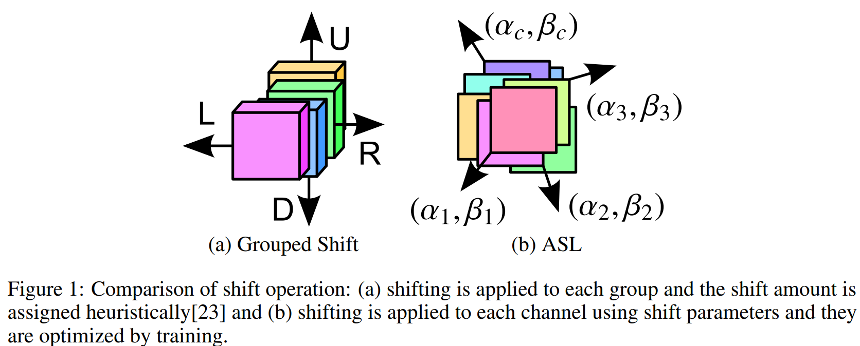
也就是將原本這篇工作中的自適應學習的偏移參數改成了固定的偏移參數.
