word2vec之tensorflow(skip-gram)實現
- 2019 年 10 月 3 日
- 筆記
關於word2vec的理解,推薦文章https://www.cnblogs.com/guoyaohua/p/9240336.html
程式碼參考https://github.com/eecrazy/word2vec_chinese_annotation
我在其基礎上修改了錯誤的部分,並添加了一些注釋。
程式碼在jupyter notebook下運行。
from __future__ import print_function #表示不管哪個python版本,使用最新的print語法  import collections  import math  import numpy as np  import random  import tensorflow as tf  import zipfile  from matplotlib import pylab
from sklearn.manifold import TSNE  %matplotlib inline
下載text8.zip文件,這個文件包含了大量單詞。官方地址為http://mattmahoney.net/dc/text8.zip
filename='text8.zip' def read_data(filename): """Extract the first file enclosed in a zip file as a list of words""" with zipfile.ZipFile(filename) as f: # 裡面只有一個文件text8,包含了多個單詞 # f.read返回位元組,tf.compat.as_str將位元組轉為字元 # data包含了所有單詞 data = tf.compat.as_str(f.read(f.namelist()[0])).split() return data #words裡面包含了所有的單詞 words = read_data(filename) print('Data size %d' % len(words))
創建正-反詞典,並將單詞轉換為詞典索引,這裡辭彙表取為50000,仍然有400000多的單詞標記為unknown。
#辭彙表大小 vocabulary_size = 50000 def build_dataset(words): # 表示未知,即不在辭彙表裡的單詞,注意這裡用的是列表形式而非元組形式,因為後面未知的數量需要賦值 count = [['UNK', -1]] count.extend(collections.Counter(words).most_common(vocabulary_size - 1)) #詞-索引哈希 dictionary = dict() for word, _ in count: # 每增加一個-->len+1,索引從0開始 dictionary[word] = len(dictionary) #用索引表示的整個text8文本 data = list() unk_count = 0 for word in words: if word in dictionary: index = dictionary[word] else: index = 0 # dictionary['UNK'] unk_count = unk_count + 1 data.append(index) count[0][1] = unk_count # 索引-詞哈希 reverse_dictionary = dict(zip(dictionary.values(), dictionary.keys())) return data, count, dictionary, reverse_dictionary data, count, dictionary, reverse_dictionary = build_dataset(words) print('Most common words (+UNK)', count[:5]) print('Sample data', data[:10]) # 刪除,減少記憶體 del words # Hint to reduce memory.
生成batch的函數
data_index = 0 # num_skips表示在兩側窗口內總共取多少個詞,數量可以小於2*skip_window # span窗口為[ skip_window target skip_window ] # num_skips=2*skip_window def generate_batch(batch_size, num_skips, skip_window): global data_index #這裡兩個斷言 assert batch_size % num_skips == 0 assert num_skips <= 2 * skip_window #初始化batch和labels,都是整形 batch = np.ndarray(shape=(batch_size), dtype=np.int32) labels = np.ndarray(shape=(batch_size, 1), dtype=np.int32) #注意labels的形狀 span = 2 * skip_window + 1 # [ skip_window target skip_window ] #buffer這個隊列太有用了,不斷地保存span個單詞在裡面,然後不斷往後滑動,而且buffer[skip_window]就是中心詞 buffer = collections.deque(maxlen=span) for _ in range(span): buffer.append(data[data_index]) data_index = (data_index + 1) % len(data) #需要多少個中心詞,因為一個target對應num_skips個的單詞,即一個目標單詞w在num_skips=2時形成2個樣本(w,left_w),(w,right_w) # 這樣描述了目標單詞w的上下文 center_words_count=batch_size // num_skips for i in range(center_words_count): #skip_window在buffer里正好是中心詞所在位置 target = skip_window # target label at the center of the buffer targets_to_avoid = [ skip_window ] for j in range(num_skips): # 選取span窗口中不包含target的,且不包含已選過的 target=random.choice([i for i in range(0,span) if i not in targets_to_avoid]) targets_to_avoid.append(target) # batch中重複num_skips次 batch[i * num_skips + j] = buffer[skip_window] # 同一個target對應num_skips個上下文單詞 labels[i * num_skips + j, 0] = buffer[target] # buffer滑動一格 buffer.append(data[data_index]) data_index = (data_index + 1) % len(data) return batch, labels # 列印前8個單詞 print('data:', [reverse_dictionary[di] for di in data[:10]]) for num_skips, skip_window in [(2, 1), (4, 2)]: data_index = 0 batch, labels = generate_batch(batch_size=16, num_skips=num_skips, skip_window=skip_window) print('nwith num_skips = %d and skip_window = %d:' % (num_skips, skip_window)) print(' batch:', [reverse_dictionary[bi] for bi in batch]) print(' labels:', [reverse_dictionary[li] for li in labels.reshape(16)])
我這裡列印的結果為:可以看到batch和label的關係為,一個target單詞多次對應於其上下文的單詞
data: ['anarchism', 'originated', 'as', 'a', 'term', 'of', 'abuse', 'first', 'used', 'against'] with num_skips = 2 and skip_window = 1: batch: ['originated', 'originated', 'as', 'as', 'a', 'a', 'term', 'term', 'of', 'of', 'abuse', 'abuse', 'first', 'first', 'used', 'used'] labels: ['as', 'anarchism', 'originated', 'a', 'term', 'as', 'of', 'a', 'term', 'abuse', 'of', 'first', 'abuse', 'used', 'against', 'first'] with num_skips = 4 and skip_window = 2: batch: ['as', 'as', 'as', 'as', 'a', 'a', 'a', 'a', 'term', 'term', 'term', 'term', 'of', 'of', 'of', 'of'] labels: ['anarchism', 'originated', 'a', 'term', 'originated', 'of', 'as', 'term', 'of', 'a', 'abuse', 'as', 'a', 'term', 'first', 'abuse']
構建model,定義loss:
batch_size = 128 embedding_size = 128 # Dimension of the embedding vector. skip_window = 1 # How many words to consider left and right. num_skips = 2 # How many times to reuse an input to generate a label. valid_size = 16 # Random set of words to evaluate similarity on. valid_window = 100 # Only pick dev samples in the head of the distribution. #隨機挑選一組單詞作為驗證集,valid_examples也就是下面的valid_dataset,是一個一維的ndarray valid_examples = np.array(random.sample(range(valid_window), valid_size)) #trick:負取樣數值 num_sampled = 64 # Number of negative examples to sample. graph = tf.Graph() with graph.as_default(), tf.device('/cpu:0'): # 訓練集和標籤,以及驗證集(注意驗證集是一個常量集合) train_dataset = tf.placeholder(tf.int32, shape=[batch_size]) train_labels = tf.placeholder(tf.int32, shape=[batch_size, 1]) valid_dataset = tf.constant(valid_examples, dtype=tf.int32) # 定義Embedding層,初始化。 embeddings = tf.Variable(tf.random_uniform([vocabulary_size, embedding_size], -1.0, 1.0)) softmax_weights = tf.Variable( tf.truncated_normal([vocabulary_size, embedding_size],stddev=1.0 / math.sqrt(embedding_size))) softmax_biases = tf.Variable(tf.zeros([vocabulary_size])) # Model. # train_dataset通過embeddings變為稠密向量,train_dataset是一個一維的ndarray embed = tf.nn.embedding_lookup(embeddings, train_dataset) # Compute the softmax loss, using a sample of the negative labels each time. # 計算損失,tf.reduce_mean和tf.nn.sampled_softmax_loss loss = tf.reduce_mean(tf.nn.sampled_softmax_loss(weights=softmax_weights, biases=softmax_biases, inputs=embed, labels=train_labels, num_sampled=num_sampled, num_classes=vocabulary_size)) # Optimizer.優化器,這裡也會優化embeddings # Note: The optimizer will optimize the softmax_weights AND the embeddings. # This is because the embeddings are defined as a variable quantity and the # optimizer's `minimize` method will by default modify all variable quantities # that contribute to the tensor it is passed. # See docs on `tf.train.Optimizer.minimize()` for more details. optimizer = tf.train.AdagradOptimizer(1.0).minimize(loss) # 模型其實到這裡就結束了,下面是在驗證集上做效果驗證 # Compute the similarity between minibatch examples and all embeddings. # We use the cosine distance:先對embeddings做正則化 norm = tf.sqrt(tf.reduce_sum(tf.square(embeddings), 1, keep_dims=True)) normalized_embeddings = embeddings / norm valid_embeddings = tf.nn.embedding_lookup(normalized_embeddings, valid_dataset) #驗證集單詞與其他所有單詞的相似度計算 similarity = tf.matmul(valid_embeddings, tf.transpose(normalized_embeddings))
開始訓練:
num_steps = 40001 with tf.Session(graph=graph) as session: tf.initialize_all_variables().run() print('Initialized') average_loss = 0 for step in range(num_steps): batch_data, batch_labels = generate_batch(batch_size, num_skips, skip_window) feed_dict = {train_dataset : batch_data, train_labels : batch_labels} _, this_loss = session.run([optimizer, loss], feed_dict=feed_dict) average_loss += this_loss # 每2000步計算一次平均loss if step % 2000 == 0: if step > 0: average_loss = average_loss / 2000 # The average loss is an estimate of the loss over the last 2000 batches. print('Average loss at step %d: %f' % (step, average_loss)) average_loss = 0 # note that this is expensive (~20% slowdown if computed every 500 steps) if step % 10000 == 0: sim = similarity.eval() for i in range(valid_size): valid_word = reverse_dictionary[valid_examples[i]] top_k = 8 # number of nearest neighbors # nearest = (-sim[i, :]).argsort()[1:top_k+1] nearest = (-sim[i, :]).argsort()[0:top_k+1]#包含自己試試 log = 'Nearest to %s:' % valid_word for k in range(top_k): close_word = reverse_dictionary[nearest[k]] log = '%s %s,' % (log, close_word) print(log) #一直到訓練結束,再對所有embeddings做一次正則化,得到最後的embedding final_embeddings = normalized_embeddings.eval()
我們可以看下訓練過程中的驗證情況,比如many這個單詞的相似詞計算:
開始時,
Nearest to many: many, originator, jeddah, maxwell, laurent, distress, interpret, bucharest,
10000步後,
Nearest to many: many, some, several, jeddah, originator, neurath, distress, songs,
40000步後,
Nearest to many: many, some, several, these, various, such, other, most,
可以看到此時單詞的相似度確實很高了。
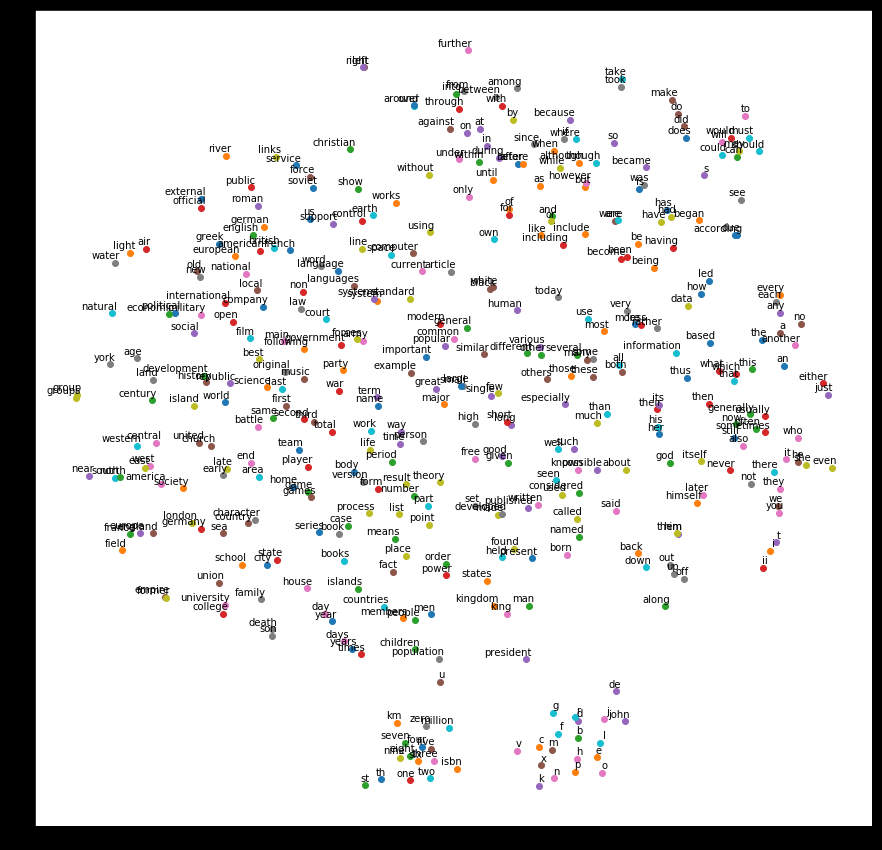
最後,我們通過降維,將單詞相似情況以圖示展現出來:
num_points = 400 # 降維度PCA tsne = TSNE(perplexity=30, n_components=2, init='pca', n_iter=5000) two_d_embeddings = tsne.fit_transform(final_embeddings[1:num_points+1, :]) def plot(embeddings, labels): assert embeddings.shape[0] >= len(labels), 'More labels than embeddings' pylab.figure(figsize=(15,15)) # in inches for i, label in enumerate(labels): x, y = embeddings[i,:] pylab.scatter(x, y) pylab.annotate(label, xy=(x, y), xytext=(5, 2), textcoords='offset points', ha='right', va='bottom') pylab.show() words = [reverse_dictionary[i] for i in range(1, num_points+1)] plot(two_d_embeddings, words)
結果如下,隨便舉些例子,university和college相近,take和took相近,one、two、three等相近
總結:原始的word2vec是用c語言寫的,這裡用的python,結合的tensorflow。這個程式碼存在一些問題,首先,單詞不是以索引作為輸入的,應該是以one-hot形式輸入。其次,負取樣的比例太小,辭彙表有50000,每批樣本才選64個去做softmax。然後,這裡也沒使用到另一個trick(當然這裡根本沒用one-hot,這個trick也不存在了,我甚至覺得根本不需要負取樣):將單詞構建為二叉樹(類似於從one-hot維度降低到二叉樹編碼(如哈夫曼樹)),從而實現一種降維操作。不過,即使是這個簡陋的模型,效果看起來依然不錯,即方向對了,醉漢也能走到家。
