機器學習——支援向量機(SVM)
- 2019 年 10 月 3 日
- 筆記
支援向量機原理
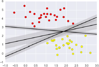
支援向量機要解決的問題其實就是尋求最優分類邊界。且最大化支援向量間距,用直線或者平面,分隔分隔超平面。
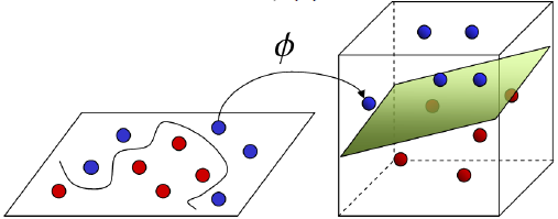
基於核函數的升維變換
通過名為核函數的特徵變換,增加新的特徵,使得低維度空間中的線性不可分問題變為高維度空間中的線性可分問題。
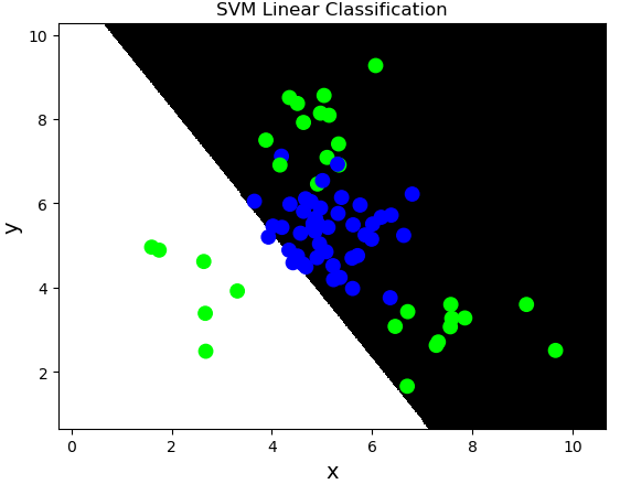
線性核函數:linear,不通過核函數進行維度提升,僅在原始維度空間中尋求線性分類邊界。
基於線性核函數的SVM分類相關API:
import sklearn.svm as svm model = svm.SVC(kernel='linear') model.fit(train_x, train_y)
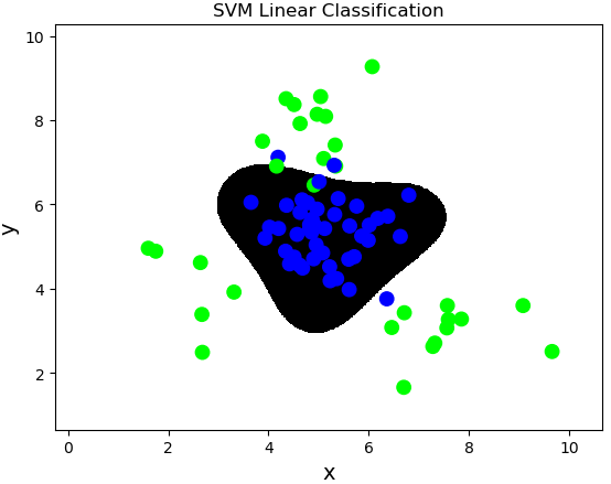
案例:對multiple2.txt中的數據進行分類。
import numpy as np import sklearn.model_selection as ms import sklearn.svm as svm import sklearn.metrics as sm import matplotlib.pyplot as mp x, y = [], [] data = np.loadtxt('../data/multiple2.txt', delimiter=',', dtype='f8') x = data[:, :-1] y = data[:, -1] train_x, test_x, train_y, test_y = ms.train_test_split(x, y, test_size=0.25, random_state=5) # 基於線性核函數的支援向量機分類器 model = svm.SVC(kernel='linear') model.fit(train_x, train_y) n = 500 l, r = x[:, 0].min() - 1, x[:, 0].max() + 1 b, t = x[:, 1].min() - 1, x[:, 1].max() + 1 grid_x = np.meshgrid(np.linspace(l, r, n), np.linspace(b, t, n)) flat_x = np.column_stack((grid_x[0].ravel(), grid_x[1].ravel())) flat_y = model.predict(flat_x) grid_y = flat_y.reshape(grid_x[0].shape) pred_test_y = model.predict(test_x) cr = sm.classification_report(test_y, pred_test_y) print(cr) mp.figure('SVM Linear Classification', facecolor='lightgray') mp.title('SVM Linear Classification', fontsize=20) mp.xlabel('x', fontsize=14) mp.ylabel('y', fontsize=14) mp.tick_params(labelsize=10) mp.pcolormesh(grid_x[0], grid_x[1], grid_y, cmap='gray') mp.scatter(test_x[:, 0], test_x[:, 1], c=test_y, cmap='brg', s=80) mp.show()
多項式核函數:poly,通過多項式函數增加原始樣本特徵的高次方冪
$$y = x_1+x_2 \
y = x_1^2 + 2x_1x_2 + x_2^2 \
y = x_1^3 + 3x_1^2x_2 + 3x_1x_2^2 + x_2^3$$
案例,基於多項式核函數訓練sample2.txt中的樣本數據。
# 基於線性核函數的支援向量機分類器 model = svm.SVC(kernel='poly', degree=3) model.fit(train_x, train_y)
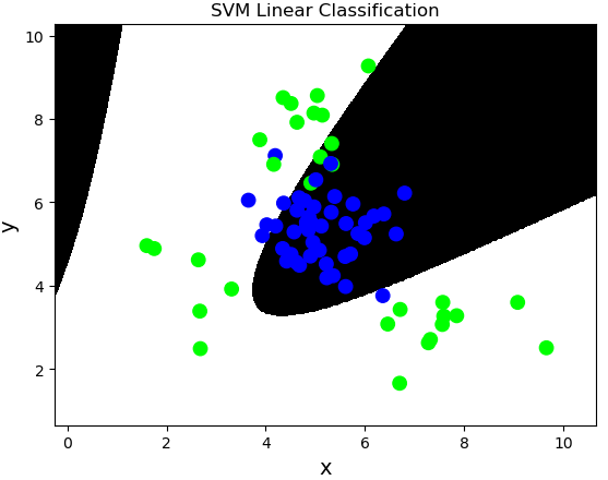
徑向基核函數:rbf,通過高斯分布函數增加原始樣本特徵的分布概率
案例,基於徑向基核函數訓練sample2.txt中的樣本數據。
# 基於徑向基核函數的支援向量機分類器 # C:正則強度 # gamma:正態分布曲線的標準差 model = svm.SVC(kernel='rbf', C=600, gamma=0.01) model.fit(train_x, train_y)
樣本類別均衡化
通過類別權重的均衡化,使所佔比例較小的樣本權重較高,而所佔比例較大的樣本權重較低,以此平均化不同類別樣本對分類模型的貢獻,提高模型性能。
樣本類別均衡化相關API:
model = svm.SVC(kernel='linear', class_weight='balanced') model.fit(train_x, train_y)
案例:修改線性核函數的支援向量機案例,基於樣本類別均衡化讀取imbalance.txt訓練模型。
... ... ... ... data = np.loadtxt('../data/imbalance.txt', delimiter=',', dtype='f8') x = data[:, :-1] y = data[:, -1] train_x, test_x, train_y, test_y = ms.train_test_split(x, y, test_size=0.25, random_state=5) # 基於線性核函數的支援向量機分類器 model = svm.SVC(kernel='linear', class_weight='balanced') model.fit(train_x, train_y) ... ... ... ...
置信概率
根據樣本與分類邊界的距離遠近,對其預測類別的可信程度進行量化,離邊界越近的樣本,置信概率越低,反之,離邊界越遠的樣本,置信概率高。
獲取每個樣本的置信概率相關API:
# 在獲取模型時,給出超參數probability=True model = svm.SVC(kernel='rbf', C=600, gamma=0.01, probability=True) 預測結果 = model.predict(輸入樣本矩陣) # 調用model.predict_proba(樣本矩陣)可以獲取每個樣本的置信概率矩陣 置信概率矩陣 = model.predict_proba(輸入樣本矩陣)
置信概率矩陣格式如下:
| 類別1 | 類別2 | |
|---|---|---|
| 樣本1 | 0.8 | 0.2 |
| 樣本2 | 0.9 | 0.1 |
| 樣本3 | 0.5 | 0.5 |
案例:修改基於徑向基核函數的SVM案例,新增測試樣本,輸出每個測試樣本的執行概率,並給出標註。
# 新增樣本 prob_x = np.array([[2, 1.5], [8, 9], [4.8, 5.2], [4, 4], [2.5, 7], [7.6, 2], [5.4, 5.9]]) pred_prob_y = model.predict(prob_x) probs = model.predict_proba(prob_x) print(probs) # [[3.00000090e-14 1.00000000e+00] # [3.00000090e-14 1.00000000e+00] # [9.73038186e-01 2.69618143e-02] # [5.65786038e-01 4.34213962e-01] # [2.77725531e-03 9.97222745e-01] # [2.91704904e-11 1.00000000e+00] # [9.43796673e-01 5.62033274e-02]] # 繪製分類邊界線 n = 500 l, r = x[:, 0].min() - 1, x[:, 0].max() + 1 b, t = x[:, 1].min() - 1, x[:, 1].max() + 1 grid_x = np.meshgrid(np.linspace(l, r, n), np.linspace(b, t, n)) flat_x = np.column_stack((grid_x[0].ravel(), grid_x[1].ravel())) flat_y = model.predict(flat_x) grid_y = flat_y.reshape(grid_x[0].shape) mp.figure('Probability', facecolor='lightgray') mp.title('Probability', fontsize=20) mp.xlabel('x', fontsize=14) mp.ylabel('y', fontsize=14) mp.tick_params(labelsize=10) mp.pcolormesh(grid_x[0], grid_x[1], grid_y, cmap='gray') mp.scatter(test_x[:, 0], test_x[:, 1], c=test_y, cmap='brg', s=80) mp.scatter(prob_x[:, 0], prob_x[:, 1], c=pred_prob_y, cmap='jet_r', s=80, marker='D') # 繪製每個測試樣本,並給出標註 for i in range(len(probs)): mp.annotate( '{}% {}%'.format( round(probs[i, 0] * 100, 2), round(probs[i, 1] * 100, 2)), xy=(prob_x[i, 0], prob_x[i, 1]), xytext=(12, -12), textcoords='offset points', horizontalalignment='left', verticalalignment='top', fontsize=9, bbox={'boxstyle': 'round,pad=0.6', 'fc': 'orange', 'alpha': 0.8}) mp.show()
網格搜索
獲取一個最優超參數的方式可以繪製驗證曲線,但是驗證曲線只能每次獲取一個最優超參數。如果多個超參數有很多排列組合的話,就可以使用網格搜索尋求最優超參數組合。
針對超參數組合列表中的每一個超參數組合,實例化給定的模型,做cv次交叉驗證,將其中平均f1得分最高的超參數組合作為最佳選擇,實例化模型對象。
網格搜索相關API:
import sklearn.model_selection as ms model = ms.GridSearchCV(模型, 超參數組合列表, cv=摺疊數) model.fit(輸入集,輸出集) # 獲取網格搜索每個參數組合 model.cv_results_['params'] # 獲取網格搜索每個參數組合所對應的平均測試分值 model.cv_results_['mean_test_score'] # 獲取最好的參數 model.best_params_ # 最優超參數組合 model.best_score_ # 最優得分 model.best_estimator_ # 最優模型對象
案例:修改置信概率案例,基於網格搜索得到最優超參數。
import numpy as np import sklearn.model_selection as ms import sklearn.svm as svm import sklearn.metrics as sm import matplotlib.pyplot as plt data = np.loadtxt('../machine_learning_date/multiple2.txt', delimiter=',', dtype='f8') x = data[:, :-1] y = data[:, -1] # 選擇svm做分類 train_x, test_x, train_y, test_y = ms.train_test_split(x, y, test_size=0.25, random_state=5) model = svm.SVC(probability=True) # 根據網格搜索選擇最優模型 # 整理網格搜索所需要的超參數列表 params = [{'kernel': ['linear'], 'C': [1, 10, 100, 1000]}, {'kernel': ['poly'], 'C': [1], 'degree': [2, 3]}, {'kernel': ['rbf'], 'C': [1, 10, 100, 1000], 'gamma': [1, 0.1, 0.01, 0.001]}] model = ms.GridSearchCV(model, params, cv=5) model.fit(train_x, train_y) # 獲取得分最優的的超參數資訊 print(model.best_params_) # {'C': 1, 'gamma': 1, 'kernel': 'rbf'} # 獲取最優得分 print(model.best_score_) # 0.96 # 獲取最優模型的資訊 print(model.best_estimator_) # SVC(C=1, cache_size=200, class_weight=None, coef0=0.0, # decision_function_shape='ovr', degree=3, gamma=1, kernel='rbf', # max_iter=-1, probability=True, random_state=None, shrinking=True, # tol=0.001, verbose=False) # 輸出每個超參數組合資訊及其得分 for param, score in zip(model.cv_results_['params'], model.cv_results_['mean_test_score']): print(param, '->', score) # {'C': 1, 'kernel': 'linear'} -> 0.5911111111111111 # {'C': 10, 'kernel': 'linear'} -> 0.5911111111111111 # ... # ... # {'C': 1000, 'gamma': 0.01, 'kernel': 'rbf'} -> 0.9555555555555556 # {'C': 1000, 'gamma': 0.001, 'kernel': 'rbf'} -> 0.92 pred_test_y = model.predict(test_x) print(sm.classification_report(test_y, pred_test_y)) # precision recall f1-score support # 0.0 0.95 0.93 0.94 45 # 1.0 0.90 0.93 0.92 30 # avg / total 0.93 0.93 0.93 75 # 新增樣本 prob_x = np.array([[2, 1.5], [8, 9], [4.8, 5.2], [4, 4], [2.5, 7], [7.6, 2], [5.4, 5.9]]) pred_prob_y = model.predict(prob_x) probs = model.predict_proba(prob_x) # 獲取每個樣本的置信概率矩陣 print(probs) # 繪製分類邊界線 n = 500 l, r = x[:, 0].min() - 1, x[:, 0].max() + 1 b, t = x[:, 1].min() - 1, x[:, 1].max() + 1 grid_x = np.meshgrid(np.linspace(l, r, n), np.linspace(b, t, n)) flat_x = np.column_stack((grid_x[0].ravel(), grid_x[1].ravel())) flat_y = model.predict(flat_x) grid_y = flat_y.reshape(grid_x[0].shape) plt.figure('Probability') plt.title('Probability') plt.xlabel('x', fontsize=14) plt.ylabel('y', fontsize=14) plt.tick_params(labelsize=10) plt.pcolormesh(grid_x[0], grid_x[1], grid_y, cmap='gray') plt.scatter(test_x[:, 0], test_x[:, 1], c=test_y, cmap='brg', s=80) plt.scatter(prob_x[:, 0], prob_x[:, 1], c=pred_prob_y, cmap='jet_r', s=80, marker='D') for i in range(len(probs)): plt.annotate('{}% {}%'.format( round(probs[i, 0] * 100, 2), round(probs[i, 1] * 100, 2)), xy=(prob_x[i, 0], prob_x[i, 1]), xytext=(12, -12), textcoords='offset points', horizontalalignment='left', verticalalignment='top', fontsize=9, bbox={'boxstyle': 'round,pad=0.6', 'fc': 'orange', 'alpha': 0.8}) plt.show()

事件預測
載入event.txt,預測某個時間段是否會出現特殊事件。
import numpy as np import sklearn.preprocessing as sp import sklearn.model_selection as ms import sklearn.svm as svm import sklearn.metrics as sm class DigitEncoder: # 模擬LabelEncoder編寫的數字編碼器 # 非數字字元串的特徵需要做標籤編碼, # 數字字元串的特徵需要做轉換編碼 def fit_transform(self, y): return y.astype('i4') def transform(self, y): return y.astype('i4') def inverse_transform(self, y): return y.astype('str') # 載入並整理數據集 # data = np.load('../machine_learning_date/events.txt', delimiter=",", dtype='U15') data = [] with open('../machine_learning_date/events.txt', 'r') as f: for line in f.readlines(): data.append(line.split(',')) data = np.array(data) data = np.delete(data, 1, axis=1) cols = data.shape[1] # 獲取一共有多少列 x, y = [], [] encoders = [] for i in range(cols): col = data[:, i] # 判斷當前列是否是數字字元串 if col[0].isdigit(): encoder = DigitEncoder() else: encoder = sp.LabelEncoder() # 使用編碼器對數據進行編碼 if i < cols - 1: x.append(encoder.fit_transform(col)) else: y = encoder.fit_transform(col) encoders.append(encoder) x = np.array(x).T # (5040,4) y = np.array(y) # (5040,) # 拆分測試集與訓練集 train_x, test_x, train_y, test_y = ms.train_test_split(x, y, test_size=0.25, random_state=7) # 構建模型 model = svm.SVC(kernel='rbf', class_weight='balanced') model.fit(train_x, train_y) # 測試 pred_test_y = model.predict(test_x) print(sm.classification_report(test_y, pred_test_y)) # 業務應用 data = [['Tuesday', '13:30:00', '21', '23']] data = np.array(data).T x = [] for row in range(len(data)): encoder = encoders[row] x.append(encoder.transform(data[row])) x = np.array(x).T pred_y = model.predict(x) print(encoders[-1].inverse_transform(pred_y)) # ['eventAn']
交通流量預測(回歸)
載入traffic.txt,預測在某個時間段某個交通路口的車流量。
"""車流量預測""" import numpy as np import sklearn.preprocessing as sp import sklearn.model_selection as ms import sklearn.svm as svm import sklearn.metrics as sm class DigitEncoder: def fit_transform(self, y): return y.astype(int) def transform(self, y): return y.astype(int) def inverse_transform(self, y): return y.astype(str) data = [] # 回歸 data = np.loadtxt('../machine_learning_date/traffic.txt', delimiter=',', dtype='U20') data = data.T encoders, x = [], [] for row in range(len(data)): if data[row][0].isdigit(): encoder = DigitEncoder() else: encoder = sp.LabelEncoder() if row < len(data) - 1: x.append(encoder.fit_transform(data[row])) else: y = encoder.fit_transform(data[row]) encoders.append(encoder) x = np.array(x).T train_x, test_x, train_y, test_y = ms.train_test_split(x, y, test_size=0.25, random_state=5) # 支援向量機回歸器 model = svm.SVR(kernel='rbf', C=10, epsilon=0.2) model.fit(train_x, train_y) pred_test_y = model.predict(test_x) print(sm.r2_score(test_y, pred_test_y)) # 0.6379517119380995 # 業務應用 data = [['Tuesday', '13:35', 'San Francisco', 'yes']] data = np.array(data).T x = [] for row in range(len(data)): encoder = encoders[row] x.append(encoder.transform(data[row])) x = np.array(x).T pred_y = model.predict(x) print(int(pred_y)) # 27
回歸:線性回歸、嶺回歸、多項式回歸、決策樹、正向激勵、隨機森林、SVR。
分類:邏輯分類、樸素貝葉斯、決策樹、隨機森林、SVC。
