基本影像操作和處理(python)

• 2019 年 10 月 3 日
• 筆記

PIL提供了通用的影像處理功能，以及大量的基本影像操作，如影像縮放、裁剪、旋轉、顏色轉換等。

Matplotlib提供了強大的繪圖功能，其下的pylab/pyplot介面包含很多方便用戶創建影像的函數。

為了觀察和進一步處理影像數據，首先需要載入影像文件，並且為了查看影像數據，我們需要將其繪製出來。

from PIL import Image  import matplotlib.pyplot as plt  import numpy as np    # 載入影像  img = Image.open("tmp.jpg")  # 轉為數組  img_data = np.array(img)  # 可視化  plt.imshow(img_data)  plt.show()

對於影像，我們常見的操作有調整影像尺寸，旋轉影像以及灰度變換

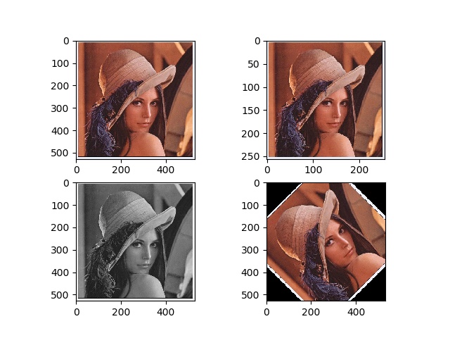
from PIL import Image  import matplotlib.pyplot as plt    img = Image.open("girl.jpg")    plt.figure()  # 子圖  plt.subplot(221)  # 原圖  plt.imshow(img)  plt.subplot(222)  # 將影像縮放至 256 * 256  plt.imshow(img.resize((256, 256)))  plt.subplot(223)  # 將影像轉為灰度圖  plt.imshow(img.convert('L'))  plt.subplot(224)  # 旋轉影像  plt.imshow(img.rotate(45))  # 保存影像  plt.savefig("tmp.jpg")  plt.show()

效果演示 ：

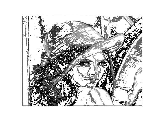
在平常的使用中，繪製影像的輪廓也經常被使用，因為繪製輪廓需要對每個坐標(x, y)的像數值施加同一個闕值，所以需要將影像灰度化

from PIL import Image  import matplotlib.pyplot as plt  import numpy as np    img = Image.open("girl.jpg")    gray_img = np.array(img.convert('L'))  plt.figure()  # 繪製影像灰度化  plt.gray()  # 關閉坐標軸  plt.axis('off')  # 繪製灰度影像  plt.contour(gray_img, origin='image')  plt.figure()  # 繪製直方圖,flatten()表示將數組展平  plt.hist(gray_img.flatten(), 128)  plt.show()  

輪廓圖及直方圖：

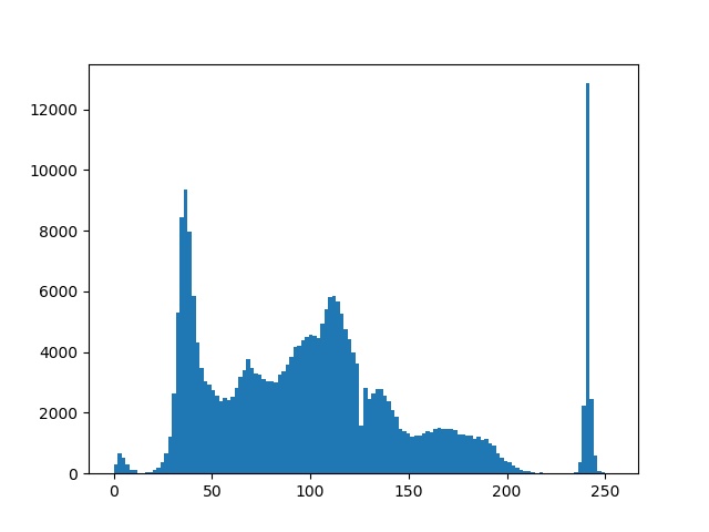
影像的直方圖用來表徵該影像的像素值的分布情況。用一定數目的小區間來指定表徵像素值的範圍，每個小區間會得到落入該小區間表示範圍的像素數目。hist()函數用於繪製影像的直方圖，其只接受一維數組作為第一個參數輸入，其第二個參數用於指定小區間的數目。

有時用戶需要和應用進行交互，如在一幅影像中標記一些點。Pylab/pyplot庫中的ginput()函數就可以實現互動式標註

from PIL import Image  import matplotlib.pyplot as plt      img = Image.open(r"girl.jpg")  plt.imshow(img)  x = plt.ginput(3)  print("clicked point: ", x)

註：該交互在集成編譯環境(pyCharm)中如果不能調出交互窗口則無法進行點擊，可以在命令窗口下成功執行。

以上我們通過numpy的array()函數將Image對象轉換成了數組，以下將展示如何從數組轉換成Image對象

from PIL import Image  import numpy as np      img = Image.open(r"girl.jpg")  img_array = np.array(img)  img = Image.fromarray(img_array)

在影像灰度變換中有一個非常有用的例子就是直方圖均衡化。直方圖均衡化是指將一幅影像的灰度直方圖變平，使變換後的影像中每個灰度值的分布概率都相同。直方圖均衡化通常是對影像灰度值進行歸一化的一個非常好的方法，並且可以增強影像的對比度。

直方圖均衡化的變換函數是影像中像素值的累積分布函數(cumulative distribution function，將像素值的範圍映射到目標範圍的歸一化操作)。

from PIL import Image  import matplotlib.pyplot as plt  import numpy as np      def histogram_equalization(img: np, nbr_bins=256):      imhist, bins = np.histogram(img.flatten())      cdf = imhist.cumsum() # 累計分布函數      # 歸一化      cdf = 255 * cdf / cdf[-1]      # 使用累積分布函數進行線性插值，計算新的像素值      img2 = np.interp(img.flatten(), bins[:-1], cdf)      return img2.reshape(img.shape), cdf      img = Image.open(r"girl.jpg").convert('L')  img2, cdf = histogram_equalization(np.array(img))  plt.figure()  plt.gray()  # 繪製子圖  plt.subplot(232)  # 變換函數  plt.plot(cdf)  plt.subplot(231)  plt.hist(np.array(img).flatten(), 256)  # 關閉坐標軸，對上一個子圖有效  plt.axis('off')  plt.subplot(233)  plt.hist(np.array(img2).flatten(), 256)  plt.axis('off')  plt.subplot(234)  plt.imshow(img)  plt.axis('off')  plt.subplot(236)  plt.imshow(img2)  plt.axis('off')  # 保存繪製影像  plt.savefig("tmp.jpg")  plt.show()    

處理結果

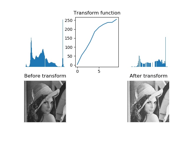
可見，直方圖均衡化的影像的對比度增強了，原先影像灰色區域的斜街變得清晰。
PCA(Principal Component Analysis, 主成分分析)是一個非常有用的降維技巧，它可以在使用儘可能少的維數的前提下，儘可能多地保持訓練數據的資訊。詳細介紹及使用見我的另一篇文章：PCA降維

SciPy是建立在Numpy基礎上，用於數值運算的開源工具包。Scipy提供很多高效的操作，可以實現數值積分、優化、統計、訊號處理，以及對我們來說最為重要的影像處理功能。

影像的高斯模糊是非常經典的影像卷積例子。本質上，影像模糊就是將(灰度)影像 (I) 和一個高斯核進行卷積操作：
[ I_sigma = I * G_sigma ]
其中， (*) 表示卷積操作；(G) 表示標準差為 (sigma) 的二維高斯核，定義為：
[ G_sigma = frac{1}{2pi sigma^2} e^{-(x^2+y^2) / 2 sigma^2} ]
高斯模糊通常是其他影像處理操作的一部分，比如影像插值操作、興趣點計算以及其他應用。

Scipy有用來做濾波操作的scipy.ndimage.filters模組。該模組使用快速一維分離的方式來計算卷積。使用方式：

from PIL import Image  import numpy as np  from scipy.ndimage import filters      img = Image.open(r"girl.jpg").convert('L')  img = np.array(img)  img2 = filters.gaussian_filter(img, 2)  img3 = filters.gaussian_filter(img, 5)  img4 = filters.gaussian_filter(img, 10)

繪製結果

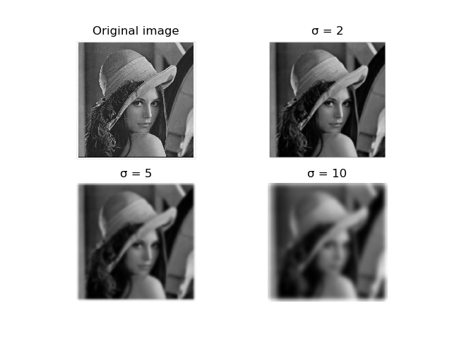
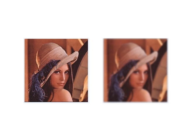
上面使用的gaussian_filter()函數中的後一個參數表示標準差 (sigma) ，可見隨著 (sigma) 的增加，影像變得越來越模糊。 (sigma) 越大，處理後影像細節丟失越多。如果是打算模糊一幅彩色影像，只需要簡單地對每一個顏色通道進行高斯模糊：

from PIL import Image  import numpy as np  from scipy.ndimage import filters      img = Image.open(r"girl.jpg")  img = np.array(img)  img2 = np.zeros(img.shape)  for i in range(img2.shape[2]):      img2[:, :, i] = filters.gaussian_filter(img[:, :, i], 5)  # 將像素值用八位表示  img2 = np.array(img2, 'uint8')

模糊結果：

在很多應用中，影像強度的變化情況是非常重要的，強度的變化可以使用灰度影像的 (x) 和 (y) 方嚮導數 (I_x) 和 (I_y)進行描述

影像的梯度向量為 (bigtriangledown I = [I_x, I_y]^T)。梯度有兩個重要屬性，一是梯度的大小：
[ | bigtriangledown I | = sqrt{I_x^2 + I_y^2} ]
它描述了影像強度變化的強弱，另一個是影像的角度：
[ alpha = arctan2(I_x, I_y) ]
它描述了影像在每個點上強度變化最大的方向。Numpy中的arctan2()函數返回弧度表示的有符號角度，角度的變化區間為 ((-pi, pi))
可以使用離散近似的方式來計算影像的導數。影像倒數大多數可以通過卷積簡單地實現：
[ I_x = I*D_x 和 I_y = I*D_y ]
對於 (D_x) 和 (D_y)，通常選擇Prewitt濾波器：
[ D_x = left[ begin{matrix} -1 & 0 & 1 \ -1 & 0 & 1 \ -1 & 0 & 1 end{matrix} right] ]
和
[ D_y = left[ begin{matrix} -1 & -1 & -1 \ 0 & 0 & 0 \ 1 & 1 & 1 end{matrix} right] ]
或者Sobel濾波器
[ D_x = left[ begin{matrix} -1 & 0 & 1 \ -2 & 0 & 2 \ -1 & 0 & 1 end{matrix} right] ]
和
[ D_y = left[ begin{matrix} -1 & -2 & -1 \ 0 & 0 & 0 \ 1 & 2 & 1 end{matrix} right] ]
這些導數濾波器可以使用scipy.ndimage.filters模組地標準卷積操作來簡單地實現

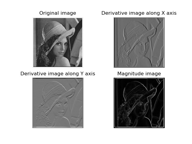
from PIL import Image  import numpy as np  from scipy.ndimage import filters      img = Image.open(r"girl.jpg").convert('L')  img = np.array(img)  imgx = np.zeros(img.shape)  # Sobel導數濾波器  filters.sobel(img, 1, imgx)    imgy = np.zeros(img.shape)  filters.sobel(img, 0, imgy)    magnitude = np.sqrt(imgx**2+imgy**2)

sobel()函數的第二個參數選擇 (x) 或 (y) 方向的導數，第三個參數保存輸出變數。在影像中，正導數顯示為亮的像素，負導數顯示為暗的像素，灰色區域表示導數的值接近零。

上面計算影像導數的方法存在缺陷：在該方法中，濾波器的尺度需要隨著影像解析度的變化而變化(?)。為了在影像雜訊方面更穩健，以及在任意尺度上計算導數，我們可以使用高斯導數濾波器：
[ I_x = I * G_{sigma x} 和 I_y = I*G_{sigma y} ]
其中，(G_{sigma x}) 和(G_{sigma y})表示(G_sigma) 在 (x) 和 (y) 方向上的導數，(G_sigma) 表示標準差為 (sigma) 的高斯函數。以下給出使用樣例：

from PIL import Image  import matplotlib.pyplot as plt  import numpy as np  from scipy.ndimage import filters    img = Image.open(r"girl.jpg").convert('L')  img = np.array(img)    sigma = 2  imgx = np.zeros(img.shape)  imgy = np.zeros(img.shape)  filters.gaussian_filter(img, (sigma, sigma), (0, 1), imgx)  filters.gaussian_filter(img, (sigma, sigma), (1, 0), imgy)    magnitude = np.sqrt(imgx**2+imgy**2)

結果演示：

在對影像進行處理時，去噪也是很重要的一環。影像去噪是在去除影像雜訊的同時，儘可能地保留影像細節和結構地處理技術，以下給出使用ROF去噪模型地Demo:

from PIL import Image  import matplotlib.pyplot as plt  import numpy as np  from scipy.ndimage import filters      def de_noise(img, U_init, tolerance=0.1, tau=0.125, tv_weight=100):      U = U_init      Px = Py = img      error = 1      while error > tolerance:          Uold = U          # 變數U梯度的x分量          gradUx = np.roll(U, -1, axis=1)-U          # 變數U梯度的y分量          gradUy = np.roll(U, -1, axis=0)-U            # 更新對偶變數          PxNew = Px + (tau/tv_weight)*gradUx          PyNew = Py + (tau/tv_weight)*gradUy          NormNew = np.maximum(1, np.sqrt(PxNew**2+PyNew**2))            # 更新x,y分量          Px = PxNew / NormNew          Py = PyNew / NormNew            # 更新原始變數          RxPx = np.roll(Px, 1, axis=1)  # 將x分量向x軸正方向平移          RyPy = np.roll(Py, 1, axis=0)  # 將y分量向y軸正方向平移            DivP = (Px - RxPx) + (Py - RyPy)  # 對偶域散度          U = img + tv_weight * DivP            error = np.linalg.norm(U - Uold)/np.sqrt(img.shape[0] * img.shape[1])            return U, img-U      if __name__ == '__main__':      im = np.zeros((500, 500))      im[100:400,100:400] = 128      im[200:300, 200:300] = 255      im = im + 30 * np.random.standard_normal((500, 500))        U, T = de_noise(im, im)      G = filters.gaussian_filter(im, 10)      plt.figure()      plt.gray()      plt.subplot(221).set_title("Original image")      plt.axis('off')      plt.imshow(im)      plt.subplot(222).set_title("Gauss blurred image")      plt.axis('off')      plt.imshow(G)      plt.subplot(223).set_title("ROF")      plt.axis('off')      plt.imshow(U)      plt.savefig('tmp.jpg')      plt.show()  

結果演示

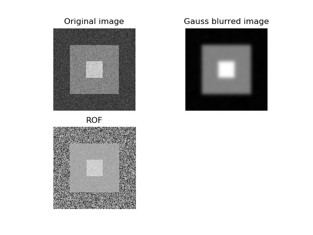
ROF去噪後的影像保留了邊緣和影像的結構資訊，同時模糊了「雜訊」。

np.roll()函數可以循環滾動元素，np.linalg.norm()用于衡量兩個數組間的差異。

之後有空將補充影像去噪

參考書籍
Python電腦視覺