Kaggle比賽(二)House Prices: Advanced Regression Techniques
- 2019 年 10 月 3 日
- 筆記
房價預測是我入門Kaggle的第二個比賽,參考學習了他人的一篇優秀教程:https://www.kaggle.com/serigne/stacked-regressions-top-4-on-leaderboard
通過Serigne的這篇notebook,我學習到了關於數據分析、特徵工程、集成學習等等很多有用的知識,在這裡感謝一下這位大佬。
本篇文章立足於Serigne的教程,將他的大部分程式碼實現了一遍,修正了個別小錯誤,也加入了自己的一些視角和思考,做了一些自認為reasonable的「改進」。最終在Leaderboard上的得分為0.11676,排名前13%。雖然最後結果反而變差了一點(沒有道理啊!QAQ),但我覺得整個實踐的過程仍然值得記錄一下。
廢話不多說,下面進入正文。
數據集概覽
導入相關Python包:
#import some necessary librairies import numpy as np # linear algebra import pandas as pd # data processing, CSV file I/O (e.g. pd.read_csv) %matplotlib inline import matplotlib.pyplot as plt # Matlab-style plotting import seaborn as sns color = sns.color_palette() sns.set_style('darkgrid') import warnings def ignore_warn(*args, **kwargs): pass warnings.warn = ignore_warn #ignore annoying warning (from sklearn and seaborn) from scipy import stats from scipy.stats import norm, skew #for some statistics pd.set_option('display.float_format', lambda x: '{:.3f}'.format(x)) #Limiting floats output to 3 decimal points from subprocess import check_output print(check_output(["ls", "../input"]).decode("utf8")) #check the files available in the directorysample_submission.csv
test.csv
train.csv
讀取csv文件:
train = pd.read_csv('datasets/train.csv') test = pd.read_csv('datasets/test.csv')查看訓練、測試集的大小:
#check the numbers of samples and features print("The train data size before dropping Id feature is : {} ".format(train.shape)) print("The test data size before dropping Id feature is : {} ".format(test.shape)) #Save the 'Id' column train_ID = train['Id'] test_ID = test['Id'] #Now drop the 'Id' colum since it's unnecessary for the prediction process. train.drop("Id", axis = 1, inplace = True) test.drop("Id", axis = 1, inplace = True) #check again the data size after dropping the 'Id' variable print("nThe train data size after dropping Id feature is : {} ".format(train.shape)) print("The test data size after dropping Id feature is : {} ".format(test.shape))The train data size before dropping Id feature is : (1460, 81)
The test data size before dropping Id feature is : (1459, 80)The train data size after dropping Id feature is : (1460, 80)
The test data size after dropping Id feature is : (1459, 79)
特徵工程
離群值處理
通過繪製散點圖可以直觀地看出特徵是否有離群值,這裡以GrLivArea為例。
fig, ax = plt.subplots() ax.scatter(x = train['GrLivArea'], y = train['SalePrice']) plt.ylabel('SalePrice', fontsize=13) plt.xlabel('GrLivArea', fontsize=13) plt.show()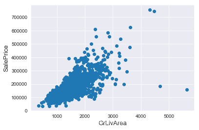
我們可以看到影像右下角的兩個點有著很大的GrLivArea,但相應的SalePrice卻異常地低,我們有理由相信它們是離群值,要將其剔除。
#Deleting outliers train = train.drop(train[(train['GrLivArea']>4000) & (train['SalePrice']<300000)].index) #Check the graphic again fig, ax = plt.subplots() ax.scatter(train['GrLivArea'], train['SalePrice']) plt.ylabel('SalePrice', fontsize=13) plt.xlabel('GrLivArea', fontsize=13) plt.show()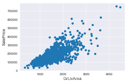
值得一提的是,刪除離群值並不總是安全的。我們不能也不必將所有的離群值全部剔除,因為測試集中依然會有一些離群值。用帶有一定雜訊的數據訓練出的模型會具有更高的魯棒性,從而在測試集中表現得更好。
目標值分析
SalePrice是我們將要預測的目標,有必要對其進行分析和處理。
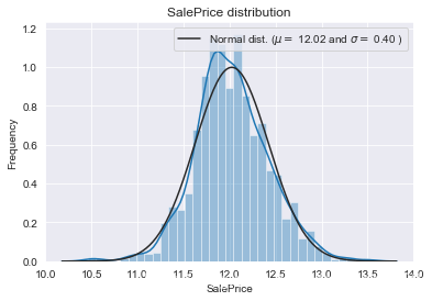
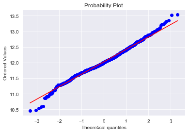
我們畫出SalePrice的分布圖和QQ圖(Quantile Quantile Plot)。這裡簡單說一下QQ圖,它是由標準正態分布的分位數為橫坐標,樣本值為縱坐標的散點圖。如果QQ圖上的點在一條直線附近,則說明數據近似於正態分布,且該直線的斜率為標準差,截距為均值。對於QQ圖的詳細介紹可以參考這篇文章:https://blog.csdn.net/hzwwpgmwy/article/details/79178485
sns.distplot(train['SalePrice'] , fit=norm); # Get the fitted parameters used by the function (mu, sigma) = norm.fit(train['SalePrice']) print( 'n mu = {:.2f} and sigma = {:.2f}n'.format(mu, sigma)) #Now plot the distribution plt.legend(['Normal dist. ($mu=$ {:.2f} and $sigma=$ {:.2f} )'.format(mu, sigma)], loc='best') plt.ylabel('Frequency') plt.title('SalePrice distribution') #Get also the QQ-plot fig = plt.figure() res = stats.probplot(train['SalePrice'], plot=plt) plt.show()mu = 180932.92 and sigma = 79467.79
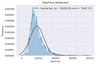
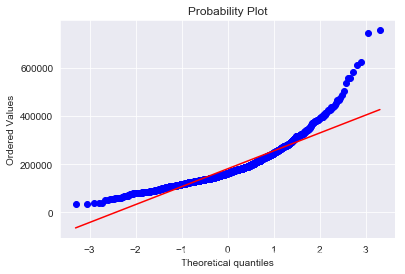
SalePrice的分布呈正偏態,而線性回歸模型要求因變數服從正態分布。我們對其做對數變換,讓數據接近正態分布。
#We use the numpy fuction log1p which applies log(1+x) to all elements of the column train["SalePrice"] = np.log1p(train["SalePrice"]) #Check the new distribution sns.distplot(train['SalePrice'] , fit=norm); # Get the fitted parameters used by the function (mu, sigma) = norm.fit(train['SalePrice']) print( 'n mu = {:.2f} and sigma = {:.2f}n'.format(mu, sigma)) #Now plot the distribution plt.legend(['Normal dist. ($mu=$ {:.2f} and $sigma=$ {:.2f} )'.format(mu, sigma)], loc='best') plt.ylabel('Frequency') plt.title('SalePrice distribution') #Get also the QQ-plot fig = plt.figure() res = stats.probplot(train['SalePrice'], plot=plt) plt.show()mu = 12.02 and sigma = 0.40
正態分布的數據有很多好的性質,使得後續的模型訓練有更好的效果。另一方面,由於這次比賽最終是對預測值的對數的誤差進行評估,所以我們在本地測試的時候也應該用同樣的標準。
特徵相關性
用相關性矩陣熱圖表現特徵與目標值之間以及兩兩特徵之間的相關程度,對特徵的處理有指導意義。
#Correlation map to see how features are correlated with SalePrice corrmat = train.corr() plt.subplots(figsize=(12,9)) sns.heatmap(corrmat, vmax=0.9, square=True)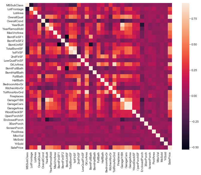
缺失值處理
首先將訓練集和測試集合併在一起:
ntrain = train.shape[0] ntest = test.shape[0] y_train = train.SalePrice.values all_data = pd.concat((train, test)).reset_index(drop=True) all_data.drop(['SalePrice'], axis=1, inplace=True) print("all_data size is : {}".format(all_data.shape))all_data size is : (2917, 79)
統計各個特徵的缺失情況:
all_data_na = (all_data.isnull().sum() / len(all_data)) * 100 all_data_na = all_data_na.drop(all_data_na[all_data_na == 0].index).sort_values(ascending=False)[:30] missing_data = pd.DataFrame({'Missing Ratio' :all_data_na}) missing_data.head(20)| Missing Ratio | |
|---|---|
| PoolQC | 99.691 |
| MiscFeature | 96.400 |
| Alley | 93.212 |
| Fence | 80.425 |
| FireplaceQu | 48.680 |
| LotFrontage | 16.661 |
| GarageQual | 5.451 |
| GarageCond | 5.451 |
| GarageFinish | 5.451 |
| GarageYrBlt | 5.451 |
| GarageType | 5.382 |
| BsmtExposure | 2.811 |
| BsmtCond | 2.811 |
| BsmtQual | 2.777 |
| BsmtFinType2 | 2.743 |
| BsmtFinType1 | 2.708 |
| MasVnrType | 0.823 |
| MasVnrArea | 0.788 |
| MSZoning | 0.137 |
| BsmtFullBath | 0.069 |
f, ax = plt.subplots(figsize=(15, 12)) plt.xticks(rotation='90') sns.barplot(x=all_data_na.index, y=all_data_na) plt.xlabel('Features', fontsize=15) plt.ylabel('Percent of missing values', fontsize=15) plt.title('Percent missing data by feature', fontsize=15)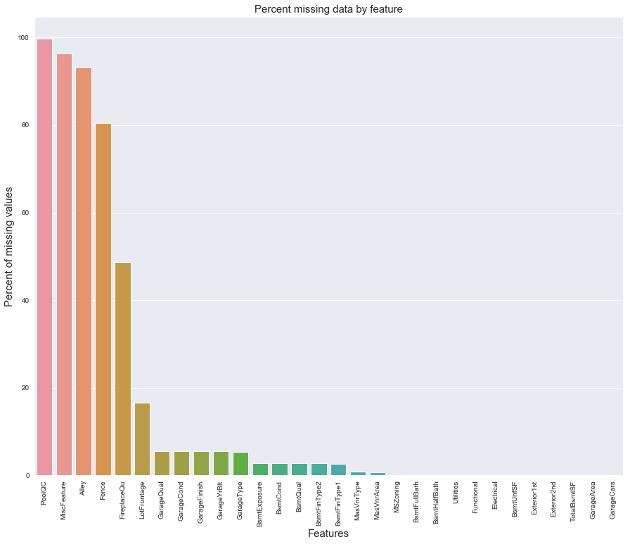
在data_description.txt中已有說明,一部分特徵值的缺失是因為這些房子根本沒有該項特徵,對於這種情況我們統一用「None」或者「0」來填充。
all_data["PoolQC"] = all_data["PoolQC"].fillna("None") all_data["MiscFeature"] = all_data["MiscFeature"].fillna("None") all_data["Alley"] = all_data["Alley"].fillna("None") all_data["Fence"] = all_data["Fence"].fillna("None") all_data["FireplaceQu"] = all_data["FireplaceQu"].fillna("None") all_data["MasVnrType"] = all_data["MasVnrType"].fillna("None") all_data["MasVnrArea"] = all_data["MasVnrArea"].fillna(0) for col in ('GarageType', 'GarageFinish', 'GarageQual', 'GarageCond'): all_data[col] = all_data[col].fillna('None') for col in ('GarageYrBlt', 'GarageArea', 'GarageCars'): all_data[col] = all_data[col].fillna(0) for col in ('BsmtFinSF1', 'BsmtFinSF2', 'BsmtUnfSF','TotalBsmtSF', 'BsmtFullBath', 'BsmtHalfBath'): all_data[col] = all_data[col].fillna(0) for col in ('BsmtQual', 'BsmtCond', 'BsmtExposure', 'BsmtFinType1', 'BsmtFinType2'): all_data[col] = all_data[col].fillna('None')對於缺失較少的離散型特徵,可以用眾數填補缺失值。
all_data['MSZoning'] = all_data['MSZoning'].fillna(all_data['MSZoning'].mode()[0]) all_data['Electrical'] = all_data['Electrical'].fillna(all_data['Electrical'].mode()[0]) all_data['KitchenQual'] = all_data['KitchenQual'].fillna(all_data['KitchenQual'].mode()[0]) all_data['Exterior1st'] = all_data['Exterior1st'].fillna(all_data['Exterior1st'].mode()[0]) all_data['Exterior2nd'] = all_data['Exterior2nd'].fillna(all_data['Exterior2nd'].mode()[0]) all_data['SaleType'] = all_data['SaleType'].fillna(all_data['SaleType'].mode()[0])對於LotFrontage項,由於每個Neighborhood的房子的LotFrontage很可能是比較相近的,所以我們可以用各個房子所在Neighborhood的LotFrontage的中位數作為填充值。
#Group by neighborhood and fill in missing value by the median LotFrontage of all the neighborhood all_data["LotFrontage"] = all_data.groupby("Neighborhood")["LotFrontage"].transform( lambda x: x.fillna(x.median()))data_description.txt中還提到過,Functional默認是「Typ」。
all_data["Functional"] = all_data["Functional"].fillna("Typ")Utilities特徵有兩個缺失值,且只有一個樣本是「NoSeWa」,除此之外全部都是「AllPub」,因此該項特徵的方差非常小,我們可以直接將其刪去。
all_data = all_data.drop(['Utilities'], axis=1)最後確認缺失值是否已全部處理完畢:
all_data.isnull().sum().max()0
進一步挖掘特徵
我們注意到有些特徵雖然是數值型的,但其實表徵的只是不同類別,其數值的大小並沒有實際意義,因此我們將其轉化為類別特徵。
all_data['MSSubClass'] = all_data['MSSubClass'].astype(str) all_data['YrSold'] = all_data['YrSold'].astype(str) all_data['MoSold'] = all_data['MoSold'].astype(str)反過來,有些類別特徵實際上有高低好壞之分,這些特徵的品質越高,就可能在一定程度導致房價越高。我們將這些特徵的類別映射成有大小的數字,以此來表徵這種潛在的偏序關係。
all_data['FireplaceQu'] = all_data['FireplaceQu'].map({'Ex': 5, 'Gd': 4, 'TA': 3, 'Fa': 2, 'Po': 1, 'None': 0}) all_data['GarageQual'] = all_data['GarageQual'].map({'Ex': 5, 'Gd': 4, 'TA': 3, 'Fa': 2, 'Po': 1, 'None': 0}) all_data['GarageCond'] = all_data['GarageCond'].map({'Ex': 5, 'Gd': 4, 'TA': 3, 'Fa': 2, 'Po': 1, 'None': 0}) all_data['GarageFinish'] = all_data['GarageFinish'].map({'Fin': 3, 'RFn': 2, 'Unf': 1, 'None': 0}) all_data['BsmtQual'] = all_data['BsmtQual'].map({'Ex': 5, 'Gd': 4, 'TA': 3, 'Fa': 2, 'Po': 1, 'None': 0}) all_data['BsmtCond'] = all_data['BsmtCond'].map({'Ex': 5, 'Gd': 4, 'TA': 3, 'Fa': 2, 'Po': 1, 'None': 0}) all_data['BsmtExposure'] = all_data['BsmtExposure'].map({'Gd': 4, 'Av': 3, 'Mn': 2, 'No': 1, 'None': 0}) all_data['BsmtFinType1'] = all_data['BsmtFinType1'].map({'GLQ': 6, 'ALQ': 5, 'BLQ': 4, 'Rec': 3, 'LwQ': 2, 'Unf': 1, 'None': 0}) all_data['BsmtFinType2'] = all_data['BsmtFinType2'].map({'GLQ': 6, 'ALQ': 5, 'BLQ': 4, 'Rec': 3, 'LwQ': 2, 'Unf': 1, 'None': 0}) all_data['ExterQual'] = all_data['ExterQual'].map({'Ex': 5, 'Gd': 4, 'TA': 3, 'Fa': 2, 'Po': 1, 'None': 0}) all_data['ExterCond'] = all_data['ExterCond'].map({'Ex': 5, 'Gd': 4, 'TA': 3, 'Fa': 2, 'Po': 1, 'None': 0}) all_data['HeatingQC'] = all_data['HeatingQC'].map({'Ex': 5, 'Gd': 4, 'TA': 3, 'Fa': 2, 'Po': 1, 'None': 0}) all_data['PoolQC'] = all_data['PoolQC'].map({'Ex': 5, 'Gd': 4, 'TA': 3, 'Fa': 2, 'Po': 1, 'None': 0}) all_data['KitchenQual'] = all_data['KitchenQual'].map({'Ex': 5, 'Gd': 4, 'TA': 3, 'Fa': 2, 'Po': 1, 'None': 0}) all_data['Functional'] = all_data['Functional'].map({'Typ': 8, 'Min1': 7, 'Min2': 6, 'Mod': 5, 'Maj1': 4, 'Maj2': 3, 'Sev': 2, 'Sal': 1, 'None': 0}) all_data['Fence'] = all_data['Fence'].map({'GdPrv': 4, 'MnPrv': 3, 'GdWo': 2, 'MnWw': 1, 'None': 0}) all_data['LandSlope'] = all_data['LandSlope'].map({'Gtl': 3, 'Mod': 2, 'Sev': 1, 'None': 0}) all_data['LotShape'] = all_data['LotShape'].map({'Reg': 4, 'IR1': 3, 'IR2': 2, 'IR3': 1, 'None': 0}) all_data['PavedDrive'] = all_data['PavedDrive'].map({'Y': 3, 'P': 2, 'N': 1, 'None': 0}) all_data['Street'] = all_data['Street'].map({'Pave': 2, 'Grvl': 1, 'None': 0}) all_data['Alley'] = all_data['Alley'].map({'Pave': 2, 'Grvl': 1, 'None': 0}) all_data['CentralAir'] = all_data['CentralAir'].map({'Y': 1, 'N': 0})利用一些重要的特徵構造更多的特徵:
all_data['TotalSF'] = all_data['TotalBsmtSF'] + all_data['1stFlrSF'] + all_data['2ndFlrSF'] all_data['OverallQual_TotalSF'] = all_data['OverallQual'] * all_data['TotalSF'] all_data['OverallQual_GrLivArea'] = all_data['OverallQual'] * all_data['GrLivArea'] all_data['OverallQual_TotRmsAbvGrd'] = all_data['OverallQual'] * all_data['TotRmsAbvGrd'] all_data['GarageArea_YearBuilt'] = all_data['GarageArea'] + all_data['YearBuilt']Box-Cox變換
對於數值型特徵,我們希望它們盡量服從正態分布,也就是不希望這些特徵出現正負偏態。
那麼我們先來計算一下各個特徵的偏度:
numeric_feats = all_data.dtypes[all_data.dtypes != "object"].index # Check the skew of all numerical features skewed_feats = all_data[numeric_feats].apply(lambda x: skew(x.dropna())).sort_values(ascending=False) skewness = pd.DataFrame({'Skew': skewed_feats}) skewness.head(10)| Skew | |
|---|---|
| MiscVal | 21.940 |
| PoolQC | 19.549 |
| PoolArea | 17.689 |
| LotArea | 13.109 |
| LowQualFinSF | 12.085 |
| 3SsnPorch | 11.372 |
| KitchenAbvGr | 4.301 |
| BsmtFinSF2 | 4.145 |
| Alley | 4.137 |
| EnclosedPorch | 4.002 |
可以看到這些特徵的偏度較高,需要做適當的處理。這裡我們對數值型特徵做Box-Cox變換,以改善數據的正態性、對稱性和方差相等性。更多關於Box-Cox變換的知識可以參考這篇部落格:https://blog.csdn.net/sinat_26917383/article/details/77864582
skewness = skewness[abs(skewness['Skew']) > 0.75] print("There are {} skewed numerical features to Box Cox transform".format(skewness.shape[0])) from scipy.special import boxcox1p skewed_features = skewness.index lam = 0.15 for feat in skewed_features: all_data[feat] = boxcox1p(all_data[feat], lam)There are 41 skewed numerical features to Box Cox transform
獨熱編碼
對於類別特徵,我們將其轉化為獨熱編碼,這樣既解決了模型不好處理屬性數據的問題,在一定程度上也起到了擴充特徵的作用。
all_data = pd.get_dummies(all_data) print(all_data.shape)(2917, 254)
現在我們有了經過處理後的訓練集和測試集:
train = all_data[:ntrain] test = all_data[ntrain:]至此,特徵工程就算完成了。
建立模型
導入演算法包:
from sklearn.linear_model import ElasticNet, Lasso from sklearn.ensemble import RandomForestRegressor, GradientBoostingRegressor from sklearn.kernel_ridge import KernelRidge from sklearn.preprocessing import RobustScaler from sklearn.base import BaseEstimator, TransformerMixin, RegressorMixin, clone from sklearn.model_selection import KFold, cross_val_score from sklearn.metrics import mean_squared_error import xgboost as xgb import lightgbm as lgb標準化
由於數據集中依然存在一定的離群點,我們首先用RobustScaler對數據進行標準化處理。
scaler = RobustScaler() train = scaler.fit_transform(train) test = scaler.transform(test)評價函數
先定義一個評價函數。我們採用5折交叉驗證。與比賽的評價標準一致,我們用Root-Mean-Squared-Error (RMSE)來為每個模型打分。
#Validation function n_folds = 5 def rmsle_cv(model): kf = KFold(n_folds, shuffle=True, random_state=42).get_n_splits(train.values) rmse= np.sqrt(-cross_val_score(model, train.values, y_train, scoring="neg_mean_squared_error", cv = kf)) return(rmse)基本模型
- 套索回歸
lasso = Lasso(alpha=0.0005, random_state=1)- 彈性網路
ENet = ElasticNet(alpha=0.0005, l1_ratio=.9, random_state=3)- 核嶺回歸
KRR = KernelRidge(alpha=0.6, kernel='polynomial', degree=2, coef0=2.5)- 梯度提升回歸
GBoost = GradientBoostingRegressor(n_estimators=1000, learning_rate=0.05, max_depth=4, max_features='sqrt', min_samples_leaf=15, min_samples_split=10, loss='huber', random_state =5)- XGBoost
model_xgb = xgb.XGBRegressor(colsample_bytree=0.5, gamma=0.05, learning_rate=0.05, max_depth=3, min_child_weight=1.8, n_estimators=1000, reg_alpha=0.5, reg_lambda=0.8, subsample=0.5, silent=1, random_state =7, nthread = -1)- LightGBM
model_lgb = lgb.LGBMRegressor(objective='regression',num_leaves=5, learning_rate=0.05, n_estimators=1000, max_bin = 55, bagging_fraction = 0.8, bagging_freq = 5, feature_fraction = 0.2, feature_fraction_seed=9, bagging_seed=9, min_data_in_leaf =6, min_sum_hessian_in_leaf = 11)看看它們的表現如何:
score = rmsle_cv(lasso) print("nLasso score: {:.4f} ({:.4f})n".format(score.mean(), score.std())) score = rmsle_cv(ENet) print("ElasticNet score: {:.4f} ({:.4f})n".format(score.mean(), score.std())) score = rmsle_cv(KRR) print("Kernel Ridge score: {:.4f} ({:.4f})n".format(score.mean(), score.std())) score = rmsle_cv(GBoost) print("Gradient Boosting score: {:.4f} ({:.4f})n".format(score.mean(), score.std())) score = rmsle_cv(model_xgb) print("Xgboost score: {:.4f} ({:.4f})n".format(score.mean(), score.std())) score = rmsle_cv(model_lgb) print("LGBM score: {:.4f} ({:.4f})n" .format(score.mean(), score.std()))Lasso score: 0.1115 (0.0073)
ElasticNet score: 0.1115 (0.0073)
Kernel Ridge score: 0.1189 (0.0045)
Gradient Boosting score: 0.1140 (0.0085)
Xgboost score: 0.1185 (0.0081)
LGBM score: 0.1175 (0.0079)
Stacking方法
集成學習往往能進一步提高模型的準確性,Stacking是其中一種效果頗好的方法,簡單來說就是學習各個基本模型的預測值來預測最終的結果。詳細步驟可參考:https://www.jianshu.com/p/59313f43916f
這裡我們用ENet、KRR和GBoost作為第一層學習器,用Lasso作為第二層學習器:
class StackingAveragedModels(BaseEstimator, RegressorMixin, TransformerMixin): def __init__(self, base_models, meta_model, n_folds=5): self.base_models = base_models self.meta_model = meta_model self.n_folds = n_folds # We again fit the data on clones of the original models def fit(self, X, y): self.base_models_ = [list() for x in self.base_models] self.meta_model_ = clone(self.meta_model) kfold = KFold(n_splits=self.n_folds, shuffle=True, random_state=156) # Train cloned base models then create out-of-fold predictions # that are needed to train the cloned meta-model out_of_fold_predictions = np.zeros((X.shape[0], len(self.base_models))) for i, model in enumerate(self.base_models): for train_index, holdout_index in kfold.split(X, y): instance = clone(model) self.base_models_[i].append(instance) instance.fit(X[train_index], y[train_index]) y_pred = instance.predict(X[holdout_index]) out_of_fold_predictions[holdout_index, i] = y_pred # Now train the cloned meta-model using the out-of-fold predictions as new feature self.meta_model_.fit(out_of_fold_predictions, y) return self #Do the predictions of all base models on the test data and use the averaged predictions as #meta-features for the final prediction which is done by the meta-model def predict(self, X): meta_features = np.column_stack([ np.column_stack([model.predict(X) for model in base_models]).mean(axis=1) for base_models in self.base_models_ ]) return self.meta_model_.predict(meta_features)Stacking的交叉驗證評分:
stacked_averaged_models = StackingAveragedModels(base_models = (ENet, GBoost, KRR), meta_model = lasso) score = rmsle_cv(stacked_averaged_models) print("Stacking Averaged models score: {:.4f} ({:.4f})".format(score.mean(), score.std()))Stacking Averaged models score: 0.1081 (0.0085)
我們得到了比單個基學習器更好的分數。
建立最終模型
我們將XGBoost、LightGBM和StackedRegressor以加權平均的方式融合在一起,建立最終的預測模型。
先定義一個評價函數:
def rmsle(y, y_pred): return np.sqrt(mean_squared_error(y, y_pred))用整個訓練集訓練模型,預測測試集的房價,並給出模型在訓練集上的評分。
- StackedRegressor
stacked_averaged_models.fit(train, y_train) stacked_train_pred = stacked_averaged_models.predict(train) stacked_pred = np.expm1(stacked_averaged_models.predict(test)) print(rmsle(y_train, stacked_train_pred))0.08464515778854238
- XGBoost
model_xgb.fit(train, y_train) xgb_train_pred = model_xgb.predict(train) xgb_pred = np.expm1(model_xgb.predict(test)) print(rmsle(y_train, xgb_train_pred))0.08362948457258125
- LightGBM
model_lgb.fit(train, y_train) lgb_train_pred = model_lgb.predict(train) lgb_pred = np.expm1(model_lgb.predict(test)) print(rmsle(y_train, lgb_train_pred))0.06344397467222622
融合模型的評分:
print('RMSLE score on train data:') print(rmsle(y_train,stacked_train_pred*0.70 + xgb_train_pred*0.15 + lgb_train_pred*0.15))RMSLE score on train data:
0.07939492590501797
預測
ensemble = stacked_pred*0.70 + xgb_pred*0.15 + lgb_pred*0.15生成提交文件
sub = pd.DataFrame() sub['Id'] = test_ID sub['SalePrice'] = ensemble sub.to_csv('submission.csv', index=False)