kaggle web traffic top solution 系列 之一
- 2021 年 1 月 4 日
- AI
首先是比賽背景介紹一下:

這個數據場景和電商的數據場景是基本差不多的,每一個page其實就是一個sku,然後後面是從2015-07-01到2017-09-10的訓練集數據,我們需要做的就是預測2017-9-13(中間gap了9-11,9-12兩天)往後63天
先總結了cpmp大佬的第二名的代碼,主要是他的代碼寫的非常簡單易懂,並且他的git代碼里使用了nn向量輸出和傳統的機器學習方法,和第一名純seq2seq的方案可以形成很好的互補,他的方案也分為多個小方案,先看一下大佬的git上寫的說明以及他在kaggle上的精彩說明。
//github.com/jfpuget/Kaggle/tree/master/WebTrafficPrediction
Kaggle上的Web流量預測競賽的2n獎解決方案。
Kaggle競爭網站:https : //www.kaggle.com/c/web-traffic-time-series-forecasting
我對競賽論壇上使用的方法作了一些說明:https : //www.kaggle.com/c/web-traffic-time-series-forecasting/discussion/39395
重現解決方案的過程:
克隆Kaggle存儲庫
將比賽數據下載到Kaggle / input目錄中
轉到Kaggle / WebTrafficPrediction目錄
運行keras-kf-12-stage2-sept-10.ipynb筆記本。這將訓練基礎深度學習模型並從中計算預測。這應該在Kaggle / submissions目錄中產生幾個文件,包括:keras_kf_12_stage2_sept_10_train.csv
keras_kf_12_stage2_sept_10_test.csv文件keras_kf_12_stage2_sept_10_test.csv是我的第一次提交。它的得分為36.91121,將整體排名第4。
運行Pred_11-stage2-sept-10.ipynb筆記本。這將創建一個基於中位數的模型並從中計算出預測。它應該在Kaggle / submissions目錄中產生文件,包括:
pred_10_stage2_sept_10_train.csv
pred_10_stage2_sept_10_test.csv運行first_stage2.ipynb筆記本。它計算頁面數據不為零的第一個日期。它應該在Kaggle / data目錄中創建一個文件:
first.csv
運行xgb_23_keras_7_2_stage2-sept-10-2.ipynb筆記本。通過在殘差上運行xgboost來創建最終模型,以進行神經網絡預測。它使用過去的訪問以及上面的兩個筆記本輸出作為功能。它應該在Kaggle / submission目錄中生成文件,包括:
xgb_1_2017-09-12-19-14-14_test.csv
該文件是我的第二次提交。它得到36.78499的分數,使我獲得第二名。
Kaggle要求提供一個更簡單的模型,以儘可能提供90%的性能。文件keras_simple.ipynb中提供了這種模型。它的功能集要簡單得多,基本上是培訓數據的最後8周中的每一個的訪問次數的中位數,加上網站(例如//es.wikipedia.org)和代理訪問方法。它的輸出得分37.58692,將獲得第9位。
這裡我們先跑一個keras-simple下的最簡單的nn模型,模型結構和複雜的nn模型是一樣的,只不過在特徵和數據方面做了一些刪減。
//www.kaggle.com/c/web-traffic-time-series-forecasting/discussion/39395
大佬的discussion內容,有點亂 我直接看代碼了….
首先是keras-simple文件里的代碼:
Python">import numpy as np
import pandas as pd
import datetime
from matplotlib import pyplot as plt
%matplotlib inline

pd.options.display.max_rows = 10
pd.options.display.max_colwidth = 100
pd.options.display.max_columns = 600
from tqdm import tqdm
import gc

from sklearn.linear_model import HuberRegressor
from sklearn.model_selection import cross_val_predict, KFold
from sklearn.decomposition import PCA

from tensorflow.keras.layers import BatchNormalization

from tensorflow.keras.models import Sequential, Model

from tensorflow.keras.layers import Input, Embedding, Dense, Activation, Dropout, Flatten

from tensorflow.keras import regularizers

from tensorflow import keras

from sklearn.preprocessing import MinMaxScaler, StandardScaler
from sklearn.model_selection import GroupKFold

def init():
    np.random.seed = 0

init()

def smape(y_true, y_pred):
    denominator = (np.abs(y_true) + np.abs(y_pred)) / 2.0
    diff = np.abs(y_true - y_pred) / denominator
    diff[denominator == 0] = 0.0
    return np.nanmean(diff)

def smape2D(y_true, y_pred):
    return smape(np.ravel(y_true), np.ravel(y_pred))

def smape_mask(y_true, y_pred, threshold):
    denominator = (np.abs(y_true) + np.abs(y_pred))
    diff = np.abs(y_true - y_pred)
    diff[denominator == 0] = 0.0

    return diff <= (threshold / 2.0) * denominator

file=r'E:\機器學習之路\機器學習比賽\web traffic'+'\\' #這個是本地的文件路徑,根據每個人存儲的
# 地方有所不同
常規的導入部分,這裡損失函數使用了smape,比賽的評價指標是smape,這裡和比賽的評估指標保持一致,不過也不一定,像最近的m5的模型訓練指標和評估指標就不是一樣的,有時候是評估指標不可微而難以直接優化,有的是因為使用其它的優化指標(目標函數)可以得到更好的效果;
max_size = 181 # number of days in 2015 with 3 days before end
offset = 1/2
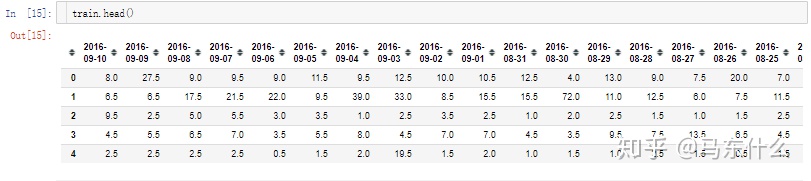
train_all = pd.read_csv(file+'train_2.csv')
train_all.head()
all_page = train_all.Page.copy()
train_key = train_all[['Page']].copy()
train_all = train_all.iloc[:,1:] * offset
train_all.head()
這裡train_key用來保存page的信息,也就是網頁的信息如上圖,後面做特徵衍生用,然後就是這裡的offset的部分,原作者對所有的原始數據進行了0.5的放縮,這裡不太明白為啥要做放縮….後面預測的時候又做了還原…醉了
def get_date_index(date, train_all=train_all):
    for idx, c in enumerate(train_all.columns):
        if date == c:
            break
    if idx == len(train_all.columns):
        return None
    return idx
定義上述函數用於確定日期的index,因為原始的數據已經進行了對齊,一行就是一個page(相當於一個電商銷量預測種的一個sku),每一個列是這個sku的銷量數據的每一天的銷量數據。

train_end = get_date_index('2016-09-10') + 1
test_start = get_date_index('2016-09-13')

train = train_all.iloc[ : , (train_end - max_size) : train_end].copy().astype('float32')
test = train_all.iloc[:, test_start : (63 + test_start)].copy().astype('float32')
train = train.iloc[:,::-1].copy().astype('float32')

train_all = train_all.iloc[:,-(max_size):].astype('float32')
train_all = train_all.iloc[:,::-1].copy().astype('float32')

test_3_date = test.columns
這裡定義了訓練集的最終日期的index和測試數據起始日的index,然後可以注意到作者僅僅取了過去的180天的數據(max_size=181)來預測未來的63天的數據,最終的數據是這樣的:

train_all是從2017-03-14到2017-09-10,
而train則是2016-03-14到2019-9-10日,
test數據集是2016年09-13到2016-11-14:

data = [page.split('_') for page in tqdm(train_key.Page)]

access = ['_'.join(page[-2:]) for page in data]

site = [page[-3] for page in data]

page = ['_'.join(page[:-3]) for page in data]
page[:2]

train_key['PageTitle'] = page
train_key['Site'] = site
train_key['AccessAgent'] = access
train_key.head()
這裡對page的特徵進行了衍生

按照page的標題、page的類型和page的代理類型衍生了3個特徵,page的特徵衍生在top1 solution中也有,不過top1做的更加細緻,把國家都弄出來了。。
這裡就是典型的靜態特徵的衍生,時間序列預測的特徵衍生方案算是常規的結構化數據的特徵衍生方案的父集,除了常規的結構化數據里會用到的特徵衍生方案之外,還有使用到時間窗、滾動平均、差分等等方式來進行時序特徵的人工表徵,這裡實際上就是結構化數據中常見的文本特徵的簡單衍生,從文本中根據先驗知識提取了一部分有意義的特徵出來。
train_norm = np.log1p(train).astype('float32')
train_norm.head()

train_all_norm = np.log1p(train_all).astype('float32')
train_all_norm.head()
對所有的價格數據進行了log1p的對數變換,常見的時序數據的標準化做法 使得原始數據的畸形程度緩解 數據之間的量綱差異大大降低,對於模型收斂幫助,關於mae mape smape的關係之前寫過:

關於標準化的問題有一些需要注意的地方:
first_day = 1 # 2016-09-13 is a Tuesday
test_columns_date = list(test.columns)
test_columns_code = ['w%d_d%d' % (i // 7, (first_day + i) % 7) for i in range(63)]
test.columns = test_columns_code

test.head()
對列名進行了簡單的修改:

test.fillna(0, inplace=True)

test['Page'] = all_page
test.sort_values(by='Page', inplace=True)
test.reset_index(drop=True, inplace=True)
對缺失值進行0填充(話說目前看到過的關於時間序列的top solution對於缺失值大部分都是直接0值處理,是缺失值的處理影響不大嗎??)然後把page放進去了,也就是每一個page的名字用於後續的merge
test = test.merge(train_key, how='left', on='Page', copy=False)

test.head()
把page衍生的特徵合併進來:

test_all_id = pd.read_csv(file+'key_2.csv')

test_all_id['Date'] = [page[-10:] for page in tqdm(test_all_id.Page)]
test_all_id['Page'] = [page[:-11] for page in tqdm(test_all_id.Page)]
test_all_id.head()
構造最終的預測數據集,讀取key的信息,然後對key文件中的page進行id和date進行分離

test_all = test_all_id.drop('Id', axis=1)
test_all['Visits_true'] = np.NaN

test_all.Visits_true = test_all.Visits_true * offset ##這句代碼沒啥意義。。。
test_all = test_all.pivot(index='Page', columns='Date', values='Visits_true').astype('float32').reset_index()

test_all['2017-11-14'] = np.NaN
test_all.sort_values(by='Page', inplace=True)
test_all.reset_index(drop=True, inplace=True)

test_all.head()
對預測用的數據集進行構造:

test_all_columns_date = list(test_all.columns[1:])
first_day = 2 # 2017-13-09 is a Wednesday
test_all_columns_code = ['w%d_d%d' % (i // 7, (first_day + i) % 7) for i in range(63)]
cols = ['Page']
cols.extend(test_all_columns_code)
test_all.columns = cols
test_all.head()
對列名進行了修改便於後續合併:

test_all = test_all.merge(train_key, how='left', on='Page')
test_all.head()
page的衍生特徵的合併
獲取標籤,
y_cols = test.columns[:63]
y_cols
test = test.reset_index()
test_all = test_all.reset_index()
test_all = test_all[test.columns].copy()
經過一系列的操作我們得到了:

其中,test_all由原來的:

變成了:

test由原來的:

變成了:

然後:
train_cols = ['d_%d' % i for i in range(train_norm.shape[1])]
train_norm.columns = train_cols
train_all_norm.columns = train_cols
將train_norm從原來的:

轉化為了:

將train_all_norm從原來的:

轉化為了:

sites = train_key.Site.unique()
test_site = pd.factorize(test.Site)[0]
test['Site_label'] = test_site
test_all['Site_label'] = test_site[:test_all.shape[0]]
accesses = train_key.AccessAgent.unique()
test_access = pd.factorize(test.AccessAgent)[0]
test['Access_label'] = test_access
test_all['Access_label'] = test_access[:test_all.shape[0]]
test0 = test.copy()
test_all0 = test_all.copy()
y_norm_cols = [c+'_norm' for c in y_cols]
y_pred_cols = [c+'_pred' for c in y_cols]
對sites和accesses進行了onehot編碼(不知道如果用embedding層會不會效果更好,類別少的時候做onehot的話,網絡設計的時候會簡單一點不用專門設置embedding再再去flatten+concat就是了)
max_periods = 16
periods = [(0,1), (1,2), (2,3), (3,4),
           (4,5), (5,6), (6,7), (7,8),
           ]


site_cols = list(sites)
access_cols = list(accesses)

for c in y_pred_cols:
    test[c] = np.NaN
    test_all[c] = np.NaN
其中,y_pred_cols是:

提前預留了要預測的結果的位置,
然後是:
test1 = add_median(test, train_norm,  ###
                   train_key, periods, max_periods, 3)

test_all1 = add_median(test_all, train_all_norm,
                       train_key, periods, max_periods, 5)
這裡的add_median的作用是對數據進行標準化處理和增加趨勢性的度量特徵,看一下這部分的代碼,注釋寫在代碼部分
# all visits is median
def add_median(test, train,
               train_key, periods, max_periods, first_train_weekday):
    train =  train.iloc[:,:7*max_periods]# 僅僅最近的7*16=112天的數據參與後面的運算

    df = train_key[['Page']].copy()
    df['AllVisits'] = train.median(axis=1).fillna(0) #這裡的AllVisits是最近的112天的訪問量的
#中位數,之所以用中位數是因為均值容易受部分極值的影響,其實使用截斷平均值也可以
    test = test.merge(df, how='left', on='Page', copy=False) #將流量的中位數合併到test數據
#集里
    test.AllVisits = test.AllVisits.fillna(0).astype('float32')# 還是簡單的0填充

    for site in sites:
        test[site] = (1 * (test.Site == site)).astype('float32') #site的onehot編碼

    for access in accesses:
        test[access] = (1 * (test.AccessAgent == access)).astype('float32')#access的onehot編碼


    for (w1, w2) in periods: #這裡periods的取值為:
#periods = [(0,1), (1,2), (2,3), (3,4),
#           (4,5), (5,6), (6,7), (7,8),
 #          ]

        df = train_key[['Page']].copy()
        d = 'median_%d_%d' % (w1, w2)
        df[d] = train.iloc[:,7*w1:7*w2].median(axis=1, skipna=True)
#計算不同周期的中為數,以(0,1)為例,這裡計算的是最近的112天中,最早的 0到7天的訪問量的中位數
# 以(1,2)為例,就是計算最近112天中,最早的7:14天的訪問量的中位數
        test = test.merge(df, how='left', on='Page', copy=False)
# 把計算出來的每一個page對應時間段下的中位數合併進來,列名為c
        test[d] = (test[d] - test.AllVisits).fillna(0).astype('float32')
# 使用c減去所有112天下的中位數,缺失值補0

    for c_norm, c in zip(y_norm_cols, y_cols):
        test[c_norm] = (np.log1p(test[c]) - test.AllVisits).astype('float32')
#使用test中的y_cols,進行log1p標準化之後減去104天的訪問量的中位數
    gc.collect()

    return test
這部分的核心代碼1:
        df[d] = train.iloc[:,7*w1:7*w2].median(axis=1, skipna=True)
#計算不同周期的中為數,以(0,1)為例,這裡計算的是最近的104天中,最早的 0到7天的訪問量的中位數
# 以(1,2)為例,就是計算最近104天中,最早的7:14天的訪問量的中位數
        test = test.merge(df, how='left', on='Page', copy=False)
# 把計算出來的每一個page對應時間段下的中位數合併進來,列名為c
        test[d] = (test[d] - test.AllVisits).fillna(0).astype('float32')
# 使用c減去所有歷史數據下的中位數,缺失值補0
這部分是典型的趨勢性特徵的衍生方法,在風控中也會有相似的處理方法,還是舉個例子吧,作者用最近的104天的數據,然後取了不同periods的時間區間:
periods = [(0,1), (1,2), (2,3), (3,4),
           (4,5), (5,6), (6,7), (7,8),
           ]
下的訪問量的中位數,用這個中位數減去104天的總的中位數來將趨勢表徵成一個特徵,比如說104天的訪問量的中位數為500,某一周的訪問量為5000,則顯然5000-500=4500是一個明顯的上述趨勢,如果某一周訪問量為0,則0-500=-500是一個明顯的下降趨勢,並且不同大小的結果可以較好的表示出趨勢的強弱,這裡也可以通過相除的方式來將趨勢性表徵出來,比如用5000/500和用0/500;
核心代碼2,也就是標準化的方法:
    for c_norm, c in zip(y_norm_cols, y_cols):
        test[c_norm] = (np.log1p(test[c]) - test.AllVisits).astype('float32')
#使用test中的y_cols,進行log1p標準化之後減去104天的訪問量的中位數
    gc.collect()
注意,這裡的ALLvisits之前已經做過log1p的變換了,這裡的test的原始的y_cols的序列數據還沒做。
所以這裡的標準化方法是,每一個page(sku)的標籤數據中的每一天,都針對於過去某個時間段的中位數進行了減法處理,畫個圖示意一下:

63天的部分,每一天的數據都減去了過去104天的訪問量的中位數,從而完成趨勢的消除,我們可以比較一下處理前後的一些page的序列的趨勢性的變化:
相對於簡單的log變換多了一個減去近期一段時間的中位數的操作,實際上本質是就是一個簡單的中位數預測+nn模型,預測的時候,兩個模型進行求和集成。
最後就是模型的構建和訓練部分了:
import keras.backend as K


group = pd.factorize(test1.Page)[0]

n_bag = 20
kf = GroupKFold(n_bag)
batch_size=4096

#print('week:', week)
test2 = test1
test_all2 = test_all1

def smape_error(y_true, y_pred):
    return K.mean(K.clip(K.abs(y_pred - y_true),  0.0, 1.0), axis=-1)


def get_model(input_dim, num_sites, num_accesses, output_dim):

    dropout = 0.5
    regularizer = 0.00004
    main_input = Input(shape=(input_dim,), dtype='float32', name='main_input')
    site_input = Input(shape=(num_sites,), dtype='float32', name='site_input')
    access_input = Input(shape=(num_accesses,), dtype='float32', name='access_input')


    x0 = keras.layers.concatenate([main_input, site_input, access_input])
    x = Dense(200, activation='relu',
              kernel_initializer='lecun_uniform', kernel_regularizer=regularizers.l2(regularizer))(x0)
    x = Dropout(dropout)(x)
    x = keras.layers.concatenate([x0, x])
    x = Dense(200, activation='relu',
              kernel_initializer='lecun_uniform', kernel_regularizer=regularizers.l2(regularizer))(x)
    x = BatchNormalization(beta_regularizer=regularizers.l2(regularizer),
                           gamma_regularizer=regularizers.l2(regularizer)
                          )(x)
    x = Dropout(dropout)(x)
    x = Dense(100, activation='relu',
              kernel_initializer='lecun_uniform', kernel_regularizer=regularizers.l2(regularizer))(x)
    x = Dropout(dropout)(x)

    x = Dense(200, activation='relu',
              kernel_initializer='lecun_uniform', kernel_regularizer=regularizers.l2(regularizer))(x)
    x = Dropout(dropout)(x)
    x = Dense(output_dim, activation='linear',
              kernel_initializer='lecun_uniform', kernel_regularizer=regularizers.l2(regularizer))(x)

    model =  Model(inputs=[main_input, site_input, access_input], outputs=[x])
    model.compile(loss=smape_error, optimizer='adam')
    return model
模型的構建如上,是一個典型的多輸入單輸出(輸出為向量)的網絡結構,關於怎麼去設計網絡結構的一些事項,可以參見百度或者谷歌上的一些煉丹手冊之類的東西,另外推薦兩本書,一本是jason brownlee的《better deep learning》簡單清晰易懂,demo+原理解釋,另外一本是《neural networks tricks of the trade》是眾學術大佬合著的一本,第二版是2018年的,相對還比較新,然後就是kaggle上的這些很不錯的網絡設計可以作為初期參考的範本。
然後是樣本的構造:
X, Xs, Xa, y = test2[num_cols].values, test2[site_cols].values, test2[access_cols].values, test2[y_norm_cols].values
X_all, Xs_all, Xa_all, y_all = test_all2[num_cols].values, test_all2[site_cols].values, test_all2[access_cols].values, test_all2[y_norm_cols].fillna(0).values

y_true = test2[y_cols]
y_all_true = test_all2[y_cols]
這裡,site_cols和access_cols都是不隨時間變化的靜態數據,動態數據僅僅使用了num_cols,num_cols為:
[‘median_0_1’,
‘median_1_2’,
‘median_2_3’,
‘median_3_4’,
‘median_4_5’,
‘median_5_6’,
‘median_6_7’,
‘median_7_8’]
根據前面的代碼:
# all visits is median
def add_median(test, train,
               train_key, periods, max_periods, first_train_weekday):
    train =  train.iloc[:,:7*max_periods]# 僅僅最近的7*16=112天的數據參與後面的運算

    df = train_key[['Page']].copy()
    df['AllVisits'] = train.median(axis=1).fillna(0) #這裡的AllVisits是最近的112天的訪問量的
#中位數,之所以用中位數是因為均值容易受部分極值的影響,其實使用截斷平均值也可以
    test = test.merge(df, how='left', on='Page', copy=False) #將流量的中位數合併到test數據
#集里
    test.AllVisits = test.AllVisits.fillna(0).astype('float32')# 還是簡單的0填充

    for site in sites:
        test[site] = (1 * (test.Site == site)).astype('float32') #site的onehot編碼

    for access in accesses:
        test[access] = (1 * (test.AccessAgent == access)).astype('float32')#access的onehot編碼


    for (w1, w2) in periods: #這裡periods的取值為:
#periods = [(0,1), (1,2), (2,3), (3,4),
#           (4,5), (5,6), (6,7), (7,8),
 #          ]

        df = train_key[['Page']].copy()
        d = 'median_%d_%d' % (w1, w2)
        df[d] = train.iloc[:,7*w1:7*w2].median(axis=1, skipna=True)
#計算不同周期的中為數,以(0,1)為例,這裡計算的是最近的112天中,最早的 0到7天的訪問量的中位數
# 以(1,2)為例,就是計算最近112天中,最早的7:14天的訪問量的中位數
        test = test.merge(df, how='left', on='Page', copy=False)
# 把計算出來的每一個page對應時間段下的中位數合併進來,列名為c
        test[d] = (test[d] - test.AllVisits).fillna(0).astype('float32')
# 使用c減去所有112天下的中位數,缺失值補0

    for c_norm, c in zip(y_norm_cols, y_cols):
        test[c_norm] = (np.log1p(test[c]) - test.AllVisits).astype('float32')
#使用test中的y_cols,進行log1p標準化之後減去112天的訪問量的中位數
    gc.collect()

    return test
我們可以知道,train部分的數據集,僅僅使用了靠近預測日期最近的112天的數據,並且更進一步的,每一周(周定義根據periods可以知道分別是1,2,3,4,5,6,7,8周)僅僅取了中位數那一天的實際流量減去112天的總的流量的中位數作為最終的動態特徵。
總的來說,就是過去112天(上圖寫錯不是104天)的最初的1~8周的流量的中位數作為動態特徵,最後是訓練部分:
group = pd.factorize(test1.Page)[0]
print(group)
n_bag = 20
kf = GroupKFold(n_bag) #這裡的網頁是完全獨立沒有任何重複,使用groupkfold和直接
#使用kfold沒有什麼區別,做了20折的交叉驗證。。。
batch_size=4096

#print('week:', week)
test2 = test1
test_all2 = test_all1


best_score = 100
best_all_score = 100


save_pred = 0
saved_pred_all = 0

for n_epoch in range(10, 201, 10):
    print('************** start %d epochs **************************' % n_epoch)

    y_pred0 = np.zeros((y.shape[0], y.shape[1])) #構建預測矩陣用於保存驗證集的預測值
    y_all_pred0 = np.zeros((n_bag, y_all.shape[0], y_all.shape[1])) #構建矩陣用於保存
#測試集的預測值
    for fold, (train_idx, test_idx) in enumerate(kf.split(X, y, group)):
        print('train fold', fold, end=' ')
        model = models[fold] #構建了20個模型,每一折訓練20個模型中的1個
        X_train, Xs_train, Xa_train, y_train = X[train_idx,:], Xs[train_idx,:], Xa[train_idx,:], y[train_idx,:]
        X_test, Xs_test, Xa_test, y_test = X[test_idx,:], Xs[test_idx,:], Xa[test_idx,:], y[test_idx,:]

        model.fit([ X_train, Xs_train, Xa_train],  y_train,
                  epochs=10, batch_size=batch_size, verbose=0, shuffle=True,
                  #validation_data=([X_test, Xs_test, Xa_test],  y_test)
                 ) #一次就跑10個epochs
        y_pred = model.predict([ X_test, Xs_test, Xa_test], batch_size=batch_size)
        y_all_pred = model.predict([X_all, Xs_all, Xa_all], batch_size=batch_size)

        y_pred0[test_idx,:] = y_pred #保存驗證集預測結果
        y_all_pred0[fold,:,:]  = y_all_pred #保存測試集預測結果

        y_pred += test2.AllVisits.values[test_idx].reshape((-1,1)) #這裡是中位數模型集成的
#部分,直接加入過去112天的流量的中位數
        y_pred = np.expm1(y_pred) #對預測結果進行還原
        y_pred[y_pred < 0.5 * offset] = 0 #預測結果小於0.5*0.5=0.25的結果直接置0
        res = smape2D(test2[y_cols].values[test_idx, :], y_pred) #計算驗證集的smape
        y_pred = offset*((y_pred / offset).round()) #預測結果進行取整。。
        res_round = smape2D(test2[y_cols].values[test_idx, :], y_pred) #取整之後的驗證集的預測
#結果的smape計算

        y_all_pred += test_all2.AllVisits.values.reshape((-1,1)) #這裡操作同上,只不過
#數據集換成了測試集
        y_all_pred = np.expm1(y_all_pred)
        y_all_pred[y_all_pred < 0.5 * offset] = 0
        res_all = smape2D(test_all2[y_cols], y_all_pred)
        y_all_pred = offset*((y_all_pred / offset).round())
        res_all_round = smape2D(test_all2[y_cols], y_all_pred)
        print('smape train: %0.5f' % res, 'round: %0.5f' % res_round,
              '     smape LB: %0.5f' % res_all, 'round: %0.5f' % res_all_round)

    #y_pred0  = np.nanmedian(y_pred0, axis=0)
    y_all_pred0  = np.nanmedian(y_all_pred0, axis=0) #預測結果取所有預測結果的中位數。。。

    y_pred0  += test2.AllVisits.values.reshape((-1,1)) #和測試集部分的操作一樣,
#對預測值進行還原,置0,smape計算等操作。。
    y_pred0 = np.expm1(y_pred0)
    y_pred0[y_pred0 < 0.5 * offset] = 0
    res = smape2D(y_true, y_pred0)
    print('smape train: %0.5f' % res, end=' ')
    y_pred0 = offset*((y_pred0 / offset).round())
    res_round = smape2D(y_true, y_pred0)
    print('round: %0.5f' % res_round)

    y_all_pred0 += test_all2.AllVisits.values.reshape((-1,1)) #同上
    y_all_pred0 = np.expm1(y_all_pred0)
    y_all_pred0[y_all_pred0 < 0.5 * offset] = 0
    #y_all_pred0 = y_all_pred0.round()
    res_all = smape2D(y_all_true, y_all_pred0)
    print('     smape LB: %0.5f' % res_all, end=' ')
    y_all_pred0 = offset*((y_all_pred0 / offset).round())
    res_all_round = smape2D(y_all_true, y_all_pred0)
    print('round: %0.5f' % res_all_round, end=' ')

    if res_round < best_score: #score的交換,如果當前循環得到的模型預測結果更好則保存
#類似於一個model的checkpoint功能
        print('saving')
        best_score = res_round
        best_all_score = res_all_round
        test.loc[:, y_pred_cols] = y_pred0 #預測結果的保存
        test_all.loc[:, y_pred_cols] = y_all_pred0
    else:
        print()
    print('*************** end %d epochs **************************' % n_epoch)
print('best saved LB score:', best_all_score)
快沒電了。。日。。。先關機了


