CTR学习笔记&代码实现2-深度ctr模型 MLP->Wide&Deep
- 2020 年 4 月 8 日
- 筆記
背景
这一篇我们从基础的深度ctr模型谈起。我很喜欢Wide&Deep的框架感觉之后很多改进都可以纳入这个框架中。Wide负责样本中出现的频繁项挖掘,Deep负责样本中未出现的特征泛化。而后续的改进要么用不同的IFC让Deep更有效的提取特征交互信息,要么是让Wide更好的记忆样本信息
Embedding + MLP
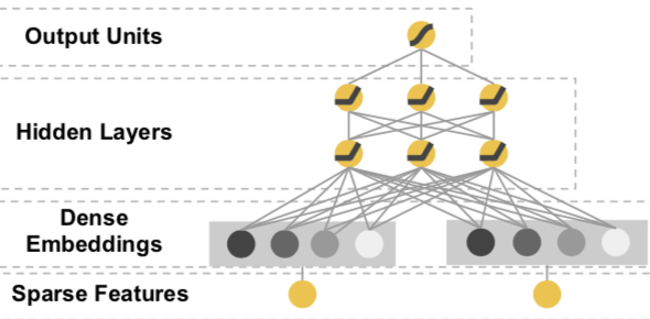
点击率模型最初在深度学习上的尝试是从简单的MLP开始的。把高维稀疏的离散特征做Embedding处理,然后把Embedding拼接作为MLP的输入,经过多层全联接神经网络的非线性变换得到对点击率的预测。
不知道你是否也像我一样困惑过,这个Embedding+MLP究竟学到了什么信息?MLP的Embedding和FM的Embedding学到的是同样的特征交互信息么?最近从大神那里听到一个蛮有说服力的观点,当然keep skeptical,欢迎一起讨论~
mlp可以学到所有特征低阶和高阶的信息表达,但依赖庞大的搜索空间。在样本有限,参数也有限的情况下往往只能学到有限的信息。因此才依赖于基于业务理解的特征工程来帮助mlp在有限的空间下学到更多有效的特征交互信息。FM的向量内积只是二阶特征工程的一种方法。之后针对deep的很多改进也是在探索如何把特征工程的业务经验用于更好的提取特征交互信息
代码实现
def build_features(numeric_handle): f_sparse = [] f_dense = [] for col, config in EMB_CONFIGS.items(): ind = tf.feature_column.categorical_column_with_hash_bucket(col, hash_bucket_size = config['hash_size']) one_hot = tf.feature_column.indicator_column(ind) f_sparse.append(one_hot) if numeric_handle == 'bucketize': # Method1 'onehot': bucket to one hot for col, config in BUCKET_CONFIGS.items(): num = tf.feature_column.numeric_column( col ) bucket = tf.feature_column.bucketized_column( num, boundaries=config ) f_sparse.append(bucket) else : # Method2 'dense': concatenate with embedding for col, config in BUCKET_CONFIGS.items(): num = tf.feature_column.numeric_column( col ) f_dense.append(num) return f_sparse, f_dense def model_fn(features, labels, mode, params): sparse_columns, dense_columns = build_features(params['numeric_handle']) with tf.variable_scope('EmbeddingInput'): embedding_input = [] for f_sparse in sparse_columns: sparse_input = tf.feature_column.input_layer(features, f_sparse) input_dim = sparse_input.get_shape().as_list()[-1] init = tf.random_normal(shape = [input_dim, params['embedding_dim']]) weight = tf.get_variable('w_{}'.format(f_sparse.name), dtype = tf.float32, initializer = init) embedding_input.append( tf.matmul(sparse_input, weight) ) dense = tf.concat(embedding_input, axis=1, name = 'embedding_concat') if params['numeric_handle'] == 'dense': numeric_input = tf.feature_column.input_layer(features, dense_columns) numeric_input = tf.layers.batch_normalization(numeric_input, center = True, scale = True, trainable =True, training = (mode == tf.estimator.ModeKeys.TRAIN)) dense = tf.concat([dense, numeric_input], axis = 1, name ='numeric_concat') with tf.variable_scope('MLP'): for i, unit in enumerate(params['hidden_units']): dense = tf.layers.dense(dense, units = unit, activation = 'relu', name = 'Dense_{}'.format(i)) if mode == tf.estimator.ModeKeys.TRAIN: add_layer_summary(dense.name, dense) dense = tf.layers.dropout(dense, rate = params['dropout_rate']) with tf.variable_scope('output'): y = tf.layers.dense(dense, units=2, activation = 'relu', name = 'output') if mode == tf.estimator.ModeKeys.PREDICT: predictions = { 'predict_class': tf.argmax(tf.nn.softmax(y), axis=1), 'prediction_prob': tf.nn.softmax(y) } return tf.estimator.EstimatorSpec(mode = tf.estimator.ModeKeys.PREDICT, predictions = predictions) cross_entropy = tf.reduce_mean(tf.nn.sparse_softmax_cross_entropy_with_logits( labels=labels, logits=y )) if mode == tf.estimator.ModeKeys.TRAIN: optimizer = tf.train.AdamOptimizer(learning_rate = params['learning_rate']) update_ops = tf.get_collection(tf.GraphKeys.UPDATE_OPS) with tf.control_dependencies(update_ops): train_op = optimizer.minimize(cross_entropy, global_step = tf.train.get_global_step()) return tf.estimator.EstimatorSpec(mode, loss = cross_entropy, train_op = train_op) else: eval_metric_ops = { 'accuracy': tf.metrics.accuracy(labels = labels, predictions = tf.argmax(tf.nn.softmax(y), axis=1)), 'auc': tf.metrics.auc(labels = labels , predictions = tf.nn.softmax(y)[:,1]), 'pr': tf.metrics.auc(labels = labels, predictions = tf.nn.softmax(y)[:,1], curve = 'PR') } return tf.estimator.EstimatorSpec(mode, loss = cross_entropy, eval_metric_ops = eval_metric_ops) Wide&Deep
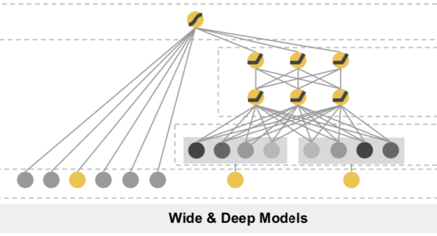
Wide&Deep是在上述MLP的基础上加入了Wide部分。作者认为Deep的部分负责generalization既样本中未出现模式的泛化和模糊查询,就是上面的Embedding+MLP。wide负责memorization既样本中已有模式的记忆,是对离散特征和特征组合做Logistics Regression。Deep和Wide一起进行联合训练。
这样说可能不完全准确,作者在文中也提到wide部分只是用来锦上添花,来帮助Deep增加那些在样本中频繁出现的模式在预测目标上的区分度。所以wide不需要是一个full-size模型,而更多需要业务上判断比较核心的特征和交叉特征。
连续特征的处理
ctr模型大多是在探讨稀疏离散特征的处理,那连续特征应该怎么处理呢?有几种处理方式
- 连续特征离散化处理,之后可以做embedding/onehot/cross
- 连续特征不做处理,直接和其他离散特征embedding后的vector拼接作为输入。这里要考虑对连续特征进行归一化处理, 不然会收敛的很慢。上面MLP尝试了BatchNorm,Wide&Deep则直接在feature_column里面做了归一化。
- 既作为连续特征输入,同时也做离散化和其他离散特征进行交互
连续特征离散化的优缺点
缺点
- 信息丢失,丢失多少信息要看桶分的咋样
- 平滑度下降,处于分桶边界的特征变动可能带来预测值比较大的波动
优点 - 加入非线性,多数情况下连续特征和目标之间都不是线性关系,而是在到达某个阈值对用户存在0/1的影响
- 更稳健,可有效避免连续特征中的极值/长尾问题
- 特征交互,做离散特征处理后方便进一步做cross特征
- 省事…,不需要再考虑啥正不正态要不要做归一化之类的
代码实现
def znorm(mean, std): def znorm_helper(col): return (col-mean)/std return znorm_helper def build_features(): f_onehot = [] f_embedding = [] f_numeric = [] # categorical features for col, config in EMB_CONFIGS.items(): ind = tf.feature_column.categorical_column_with_hash_bucket(col, hash_bucket_size = config['hash_size']) f_onehot.append( tf.feature_column.indicator_column(ind)) f_embedding.append( tf.feature_column.embedding_column(ind, dimension = config['emb_size']) ) # numeric features: both in numeric feature and bucketized to discrete feature for col, config in BUCKET_CONFIGS.items(): num = tf.feature_column.numeric_column(col, normalizer_fn = znorm(NORM_CONFIGS[col]['mean'],NORM_CONFIGS[col]['std'] )) f_numeric.append(num) bucket = tf.feature_column.bucketized_column( num, boundaries=config ) f_onehot.append(bucket) # crossed features for col1,col2 in combinations(f_onehot,2): # if col is indicator of hashed bucuket, use raw feature directly if col1.parents[0].name in EMB_CONFIGS.keys(): col1 = col1.parents[0].name if col2.parents[0].name in EMB_CONFIGS.keys(): col2 = col2.parents[0].name crossed = tf.feature_column.crossed_column([col1, col2], hash_bucket_size = 20) f_onehot.append(tf.feature_column.indicator_column(crossed)) f_dense = f_embedding + f_numeric #f_dense = f_embedding + f_numeric + f_onehot f_sparse = f_onehot #f_sparse = f_onehot + f_numeric return f_sparse, f_dense def build_estimator(model_dir): sparse_feature, dense_feature= build_features() run_config = tf.estimator.RunConfig( save_summary_steps=50, log_step_count_steps=50, keep_checkpoint_max = 3, save_checkpoints_steps =50 ) dnn_optimizer = tf.train.ProximalAdagradOptimizer( learning_rate= 0.001, l1_regularization_strength=0.001, l2_regularization_strength=0.001 ) estimator = tf.estimator.DNNLinearCombinedClassifier( model_dir=model_dir, linear_feature_columns=sparse_feature, dnn_feature_columns=dense_feature, dnn_optimizer = dnn_optimizer, dnn_dropout = 0.1, batch_norm = False, dnn_hidden_units = [48,32,16], config=run_config ) return estimator 完整代码在这里 https://github.com/DSXiangLi/CTR
CTR学习笔记&代码实现系列?
CTR学习笔记&代码实现1-深度学习的前奏LR->FFM
参考材料
- Weinan Zhang, Tianming Du, and Jun Wang. Deep learning over multi-field categorical data – – A case study on user response prediction. In ECIR, 2016.
- Cheng H T, Koc L, Harmsen J, et al. Wide & deep learning for recommender systems[C]//Proceedings of the 1st Workshop on Deep Learning for Recommender Systems. ACM, 2016: 7-10
- https://www.jiqizhixin.com/articles/2018-07-16-17
- https://cloud.tencent.com/developer/article/1063010
- https://github.com/shenweichen/DeepCTR