机器学习——分类问题
- 2019 年 10 月 3 日
- 筆記
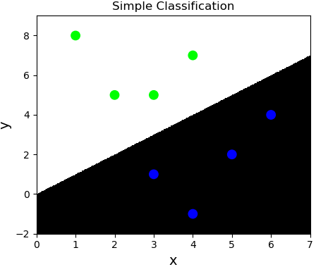
人工分类
特征1>特征2 输出 0
特征1<特征2 输出 1
| 特征1 | 特征2 | 输出 |
|---|---|---|
| 3 | 1 | 0 |
| 2 | 5 | 1 |
| 1 | 8 | 1 |
| 6 | 4 | 0 |
| 5 | 2 | 0 |
| 3 | 5 | 1 |
| 4 | 7 | 1 |
| 4 | -1 | 0 |
| … | … | … |
| 6 | 8 | 1 |
| 5 | 1 | 0 |
案例:
import numpy as np import matplotlib.pyplot as plt x = np.array([[3, 1], [2, 5], [1, 8], [6, 4], [5, 2], [3, 5], [4, 7], [4, -1]]) y = np.array([0, 1, 1, 0, 0, 1, 1, 0]) # 把整个空间分为500*500的网格化矩阵 l, r = x[:, 0].min() - 1, x[:, 0].max() + 1 # 横轴最小、最大 b, t = x[:, 1].min() - 1, x[:, 1].max() + 1 # 纵轴最小、最大 grid_x, grid_y = np.meshgrid(np.linspace(l, r, 500), np.linspace(b, t, 500)) # grid_z存储了网格化矩阵中每个坐标点的类别标签:0 / 1 grid_z = np.piecewise(grid_x, [grid_x > grid_y, grid_x < grid_y], [0, 1]) # 绘制散点图 plt.figure('Simple Classification', facecolor='lightgray') plt.title('Simple Classification', fontsize=20) plt.xlabel('x', fontsize=14) plt.ylabel('y', fontsize=14) plt.tick_params(labelsize=10) # 为网格化矩阵中的每个元素填充背景颜色 plt.pcolormesh(grid_x, grid_y, grid_z, cmap='gray') plt.scatter(x[:, 0], x[:, 1], c=y, cmap='brg', s=80) plt.show()
逻辑分类
通过输入的样本数据,基于多元线型回归模型求出线性预测方程。
$$y=w_0+w_1x_1+w_2x_2$$
但通过线型回归方程返回的是连续值,不可以直接用于分类业务模型,所以急需一种方式使得把连续的预测值->离散的预测值。 [-oo, +oo]->{0, 1}
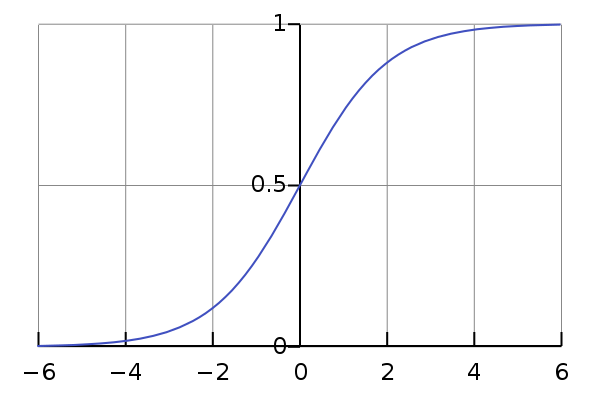
sigmoid函数当x>0,y>0.5;当x<0, y<0.5; 可以把样本数据经过线性预测模型求得的值带入逻辑函数的x,即将预测函数的输出看做输入被划分为1类的概率,概率大的类别作为预测结果,可以根据函数值确定两个分类。这是连续函数离散化的一种方式。
逻辑回归相关API:
import sklearn.linear_model as lm # 构建逻辑回归器 model = lm.LogisticRegression(solver='liblinear', C=正则强度) # solver:逻辑函数中指数的函数关系(liblinear为线型函数关系) # C:正则化系数λ的倒数,为了防止过拟合。越小的数值表示越强的正则化。 model.fit(输入, 输出) result = model.predict(待预测的值)
案例:基于逻辑回归器绘制网格化坐标颜色矩阵。
import numpy as np import matplotlib.pyplot as plt import sklearn.linear_model as lm x = np.array([[4, 7], [3.5, 8], [3.1, 6.2], [0.5, 1], [1, 2], [1.2, 1.9], [6, 2], [5.7, 1.5], [5.4, 2.2]]) y = np.array([0, 0, 0, 1, 1, 1, 2, 2, 2]) # 3个类别 # 把整个空间分为500*500的网格化矩阵 l, r = x[:, 0].min() - 1, x[:, 0].max() + 1 b, t = x[:, 1].min() - 1, x[:, 1].max() + 1 grid_x, grid_y = np.meshgrid(np.linspace(l, r, 500), np.linspace(b, t, 500)) # 把grid_x与grid_y变成一维,并在一起成两列,作为测试集x mesh_x = np.column_stack((grid_x.ravel(), grid_y.ravel())) # 创建模型,针对test_x预测相应输出 model = lm.LogisticRegression(solver='liblinear', C=200) model.fit(x, y) mesh_y = model.predict(mesh_x) # 把预测结果变维:500*500,用于绘制分类边界线 grid_z = mesh_y.reshape(grid_x.shape) # 绘制散点图 plt.figure('Simple Classification') plt.title('Simple Classification') plt.xlabel('x', fontsize=14) plt.ylabel('y', fontsize=14) plt.tick_params(labelsize=10) # 为网格化矩阵中的每个元素填充背景颜色 plt.pcolormesh(grid_x, grid_y, grid_z, cmap='gray') plt.scatter(x[:, 0], x[:, 1], c=y, cmap='brg', s=80) plt.show()

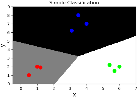
多元分类
通过多个二元分类器解决多元分类问题。
| 特征1 | 特征2 | ==> | 所属类别 |
|---|---|---|---|
| 4 | 7 | ==> | A |
| 3.5 | 8 | ==> | A |
| 1.2 | 1.9 | ==> | B |
| 5.4 | 2.2 | ==> | C |
若拿到一组新的样本,可以基于二元逻辑分类训练出一个模型判断属于A类别的概率。再使用同样的方法训练出两个模型分别判断属于B、C类型的概率,最终选择概率最高的类别作为新样本的分类结果。
案例:基于逻辑分类模型的多元分类。
import numpy as np import matplotlib.pyplot as plt import sklearn.linear_model as lm x = np.array([[4, 7], [3.5, 8], [3.1, 6.2], [0.5, 1], [1, 2], [1.2, 1.9], [6, 2], [5.7, 1.5], [5.4, 2.2]]) y = np.array([0, 0, 0, 1, 1, 1, 2, 2, 2]) # 把整个空间分为500*500的网格化矩阵 l, r = x[:, 0].min() - 1, x[:, 0].max() + 1 b, t = x[:, 1].min() - 1, x[:, 1].max() + 1 grid_x, grid_y = np.meshgrid(np.linspace(l, r, 500), np.linspace(b, t, 500)) # 把grid_x与grid_y变成一维,并在一起成两列,作为测试集x mesh_x = np.column_stack((grid_x.ravel(), grid_y.ravel())) # 创建模型,针对test_x预测相应输出 model = lm.LogisticRegression(solver='liblinear', C=200) model.fit(x, y) mesh_y = model.predict(mesh_x) # 把预测结果变维:500*500,用于绘制分类边界线 grid_z = mesh_y.reshape(grid_x.shape) # 绘制散点图 plt.figure('Simple Classification', facecolor='lightgray') plt.title('Simple Classification', fontsize=20) plt.xlabel('x', fontsize=14) plt.ylabel('y', fontsize=14) plt.tick_params(labelsize=10) # 为网格化矩阵中的每个元素填充背景颜色 plt.pcolormesh(grid_x, grid_y, grid_z, cmap='gray') plt.scatter(x[:, 0], x[:, 1], c=y, cmap='brg', s=80) plt.show()
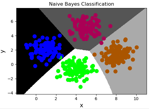
朴素贝叶斯分类
朴素贝叶斯分类是一种依据统计概率理论而实现的一种分类方式。观察这组数据:
| 天气情况 | 穿衣风格 | 约女朋友 | ==> | 心情 |
|---|---|---|---|---|
| 0(晴天) | 0(休闲) | 0(约了) | ==> | 0(高兴) |
| 0 | 1(风骚) | 1(没约) | ==> | 0 |
| 1(多云) | 1 | 0 | ==> | 0 |
| 0 | 2(破旧) | 1 | ==> | 1(郁闷) |
| 2(下雨) | 2 | 0 | ==> | 0 |
| … | … | … | ==> | … |
| 0 | 1 | 0 | ==> | ? |
通过上述训练样本如何预测:晴天、穿着风骚、还约女朋友时的心情?可以整理相同特征值的样本,计算属于某类别的概率即可。但是如果在样本空间没有完全匹配的数据该如何预测?
贝叶斯定理:P(A|B)=P(B|A)P(A)/P(B) <== P(A, B) = P(A) P(B|A) = P(B) P(A|B)
例如:
假设一个学校里有60%男生和4 0%女生.女生穿裤子的人数和穿裙子的人数相等,所有男生穿裤子. 一个人在远处随机看到了一个穿裤子的学生.那么这个学生是女生的概率是多少?
P(女) = 0.4
P(裤子|女) = 0.5
P(裤子) = 0.6 + 0.2 = 0.8
P(女|裤子) = P(裤子|女) * P(女) / P(裤子) = 0.5 * 0.4 / 0.8 = 0.25
根据贝叶斯定理,如何预测:晴天、穿着休闲、没有约女朋友时的心情?
P(晴天,休闲,没约,高兴)
= P(晴天|休闲,没约,高兴) P(休闲,没约,高兴)
= P(晴天|休闲,没约,高兴) P(休闲|没约,高兴) P(没约,高兴)
= P(晴天|休闲,没约,高兴) P(休闲|没约,高兴) P(没约|高兴)P(高兴)
( 朴素:条件独立,特征值之间没有因果关系)
休闲条件下晴天的概率和没约条件下晴天的概率,相互独立,因此概率相等。
= P(晴天|高兴) P(休闲|高兴) P(没约|高兴)P(高兴)
由此可得,统计总样本空间中晴天、穿着休闲、没有约女朋友时高兴的概率,与晴天、穿着休闲、没有约女朋友时不高兴的概率,择其大者为最终结果。
高斯贝叶斯分类器相关API:
import sklearn.naive_bayes as nb model = nb.GaussianNB() # 创建高斯分布朴素贝叶斯分类器 model.fit(x, y) result = model.predict(samples)
案例(multip.txt):
import sklearn.naive_bayes as nb import numpy as np import matplotlib.pyplot as plt data = np.loadtxt('../machine_learning_date/multiple1.txt', delimiter=',', usecols=(0, 1, 2), unpack=False) print(data.shape) # (400, 3) x = data[:, :2] y = data[:, 2] model = nb.GaussianNB() # 创建高斯朴素贝叶斯分类器 model.fit(x, y) # 绘制背景颜色,显示分类边界线 # 把整个空间分为500*500的网格化矩阵 l, r = x[:, 0].min() - 1, x[:, 0].max() + 1 b, t = x[:, 1].min() - 1, x[:, 1].max() + 1 grid_x, grid_y = np.meshgrid(np.linspace(l, r, 500), np.linspace(b, t, 500)) # 把grid_x与grid_y抻平并在一起成两列,作为测试集x mesh_x = np.column_stack((grid_x.ravel(), grid_y.ravel())) mesh_y = model.predict(mesh_x) grid_z = mesh_y.reshape(grid_x.shape) # 把所有样本点都绘制出来 plt.figure('Naive Bayes Classification', facecolor='lightgray') plt.title('Naive Bayes Classification', fontsize=20) plt.xlabel('x', fontsize=14) plt.ylabel('y', fontsize=14) plt.tick_params(labelsize=10) plt.pcolormesh(grid_x, grid_y, grid_z, cmap='gray') plt.scatter(x[:, 0], x[:, 1], c=y, cmap='brg', s=80) plt.show()
数据集划分
对于分类问题训练集和测试集的划分不应该用整个样本空间的特定百分比作为训练数据,而应该在其每一个类别的样本中抽取特定百分比作为训练数据。sklearn模块提供了数据集划分相关方法,可以方便的划分训练集与测试集数据,使用不同数据集训练或测试模型,达到提高分类可信度。
数据集划分相关API:
import sklearn.model_selection as ms 训练输入, 测试输入, 训练输出, 测试输出 = ms.train_test_split(输入集, 输出集, test_size=测试集占比, random_state=随机种子)
案例:
import numpy as np import sklearn.model_selection as ms import sklearn.naive_bayes as nb import matplotlib.pyplot as mp data = np.loadtxt('../machine_learning_data/multiple1.txt', unpack=False, dtype='U20', delimiter=',') print(data.shape) x = np.array(data[:, :-1], dtype=float) y = np.array(data[:, -1], dtype=float) # 划分训练集和测试集 train_x, test_x, train_y, test_y = ms.train_test_split( x, y, test_size=0.25, random_state=7) # 朴素贝叶斯分类器 model = nb.GaussianNB() # 用训练集训练模型 model.fit(train_x, train_y) l, r = x[:, 0].min() - 1, x[:, 0].max() + 1 b, t = x[:, 1].min() - 1, x[:, 1].max() + 1 n = 500 grid_x, grid_y = np.meshgrid(np.linspace(l, r, n), np.linspace(b, t, n)) samples = np.column_stack((grid_x.ravel(), grid_y.ravel())) grid_z = model.predict(samples) grid_z = grid_z.reshape(grid_x.shape) pred_test_y = model.predict(test_x) # 计算并打印预测输出的精确度 print((test_y == pred_test_y).sum() / pred_test_y.size) mp.figure('Naive Bayes Classification', facecolor='lightgray') mp.title('Naive Bayes Classification', fontsize=20) mp.xlabel('x', fontsize=14) mp.ylabel('y', fontsize=14) mp.tick_params(labelsize=10) mp.pcolormesh(grid_x, grid_y, grid_z, cmap='gray') mp.scatter(test_x[:,0], test_x[:,1], c=test_y, cmap='brg', s=80) mp.show()
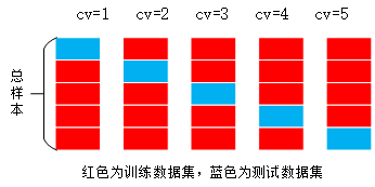
交叉验证
由于数据集的划分有不确定性,若随机划分的样本正好处于某类特殊样本,则得到的训练模型所预测的结果的可信度将受到质疑。所以需要进行多次交叉验证,把样本空间中的所有样本均分成n份,使用不同的训练集训练模型,对不同的测试集进行测试时输出指标得分。
sklearn提供了交叉验证相关API:
import sklearn.model_selection as ms ms.cross_val_score(模型, 输入集, 输出集, cv=折叠数, scoring=指标名)->指标值数组
案例:使用交叉验证,输出分类器的精确度:
# 划分测试集与训练集 train_x, test_x, train_y, test_y = ms.train_test_split(x, y, test_size=0.25, random_state=7) model = nb.GaussianNB() # 创建并且训练模型 # 精确度 ac = ms.cross_val_score(model, train_x, train_y, cv=5, scoring='accuracy') print(ac.mean()) # 0.9966101694915255 model.fit(train_x, train_y)
交叉验证指标
-
精确度(accuracy):分类正确的样本数/总样本数
-
查准率(precision_weighted):针对每一个类别,预测正确的样本数比上预测出来的样本数
-
召回率(recall_weighted):针对每一个类别,预测正确的样本数比上实际存在的样本数
-
f1得分(f1_weighted):$frac{2*查准率*召回率}{查准率+召回率}$
在交叉验证过程中,针对每一次交叉验证,计算所有类别的查准率、召回率或者f1得分,然后取各类别相应指标值的平均数,作为这一次交叉验证的评估指标,然后再将所有交叉验证的评估指标以数组的形式返回调用者。
# 精确度 ac = ms.cross_val_score( model, train_x, train_y, cv=5, scoring='accuracy') print(ac.mean()) # 查准率 pw = ms.cross_val_score( model, train_x, train_y, cv=5, scoring='precision_weighted') print(pw.mean()) # 召回率 rw = ms.cross_val_score( model, train_x, train_y, cv=5, scoring='recall_weighted') print(rw.mean()) # f1得分 fw = ms.cross_val_score( model, train_x, train_y, cv=5, scoring='f1_weighted') print(fw.mean())
混淆矩阵
每一行和每一列分别对应样本输出中的每一个类别,行表示实际类别,列表示预测类别。
| A类别 | B类别 | C类别 | |
|---|---|---|---|
| A类别 | 5 | 0 | 0 |
| B类别 | 0 | 6 | 0 |
| C类别 | 0 | 0 | 7 |
上述矩阵即为理想的混淆矩阵。不理想的混淆矩阵如下:
| A类别 | B类别 | C类别 | |
|---|---|---|---|
| A类别 | 3 | 1 | 1 |
| B类别 | 0 | 4 | 2 |
| C类别 | 0 | 0 | 7 |
$查准率 = frac{主对角线上的值}{该值所在列的和}$
$召回率 = frac{主对角线上的值}{该值所在行的和}$
获取模型分类结果的混淆矩阵的相关API:
import sklearn.metrics as sm sm.confusion_matrix(实际输出, 预测输出)
案例:输出分类结果的混淆矩阵。
# 输出混淆矩阵 cm = sm.confusion_matrix(test_y, pred_test_y) print(cm) # [[22 0 0 0] # [ 0 27 1 0] # [ 0 0 25 0] # [ 0 0 0 25]] plt.imshow(cm, cmap='gray') plt.show()
分类报告
sklearn.metrics提供了分类报告相关API,不仅可以得到混淆矩阵,还可以得到交叉验证查准率、召回率、f1得分和每个标签出现的次数的结果,可以方便的分析出哪些样本是异常样本。
# 获取分类报告 cr = sm.classification_report(实际输出, 预测输出)
案例:输出分类报告:
# 输出分类报告 cr = sm.classification_report(test_y, pred_test_y) print(cr) # precision recall f1-score support # # 0.0 1.00 1.00 1.00 22 # 1.0 1.00 0.96 0.98 28 # 2.0 0.96 1.00 0.98 25 # 3.0 1.00 1.00 1.00 25 # # avg / total 0.99 0.99 0.99 100
决策树分类
决策树分类模型会找到与样本特征匹配的叶子节点然后以投票的方式进行分类。在样本文件中统计了小汽车的常见特征信息及小汽车的分类,使用这些数据基于决策树分类算法训练模型预测小汽车等级。
| 汽车价格 | 维修费用 | 车门数量 | 载客数 | 后备箱 | 安全性 | 汽车级别 |
|---|
案例:基于决策树分类算法训练模型预测小汽车等级。car.txt数据集
1、读取文本数据,对每列进行标签编码,基于随机森林分类器进行模型训练,进行交叉验证。
import numpy as np import sklearn.preprocessing as sp import sklearn.ensemble as se import sklearn.model_selection as ms def f(s): return str(s, encoding='utf-8') # 读取文件 data = np.loadtxt('../machine_learning_date/car.txt', delimiter=',', dtype='U20', converters={0: f, 1: f, 2: f, 3: f, 4: f, 5: f, 6: f}) # 整理训练集的输入与输出 data = data.T train_x, train_y = [], [] encoders = [] for col in range(len(data)): lbe = sp.LabelEncoder() # 标签编码 if col < len(data) - 1: # 不是最后一列 train_x.append(lbe.fit_transform(data[col])) else: train_y = lbe.fit_transform(data[col]) encoders.append(lbe) # 保存每列的标签编码器 train_x = np.array(train_x).T print(train_x) # [[3 3 0 0 2 1] # [3 3 0 0 2 2] # [3 3 0 0 2 0] # ... # [1 1 3 2 0 1] # [1 1 3 2 0 2] # [1 1 3 2 0 0]] # 创建随机森林分类器 model = se.RandomForestClassifier(max_depth=6, n_estimators=200, random_state=7) # 交叉验证 cv = ms.cross_val_score(model, train_x, train_y, cv=5, scoring='f1_weighted') model.fit(train_x, train_y)
2、自定义测试集,使用已训练的模型对测试集进行测试,输出结果。
# 模型测试 data = [ ['high', 'med', '5more', '4', 'big', 'low', 'unacc'], ['high', 'high', '4', '4', 'med', 'med', 'acc'], ['low', 'low', '2', '4', 'small', 'high', 'good'], ['low', 'med', '3', '4', 'med', 'high', 'vgood']] # 在训练时需要把所有的LabelEncoder保存下来, # 在测试时,对测试数据的每一列使用相同的编码器进行编码, # 然后进行预测,得出预测结果 data = np.array(data).T test_x, test_y = [], [] for col in range(len(data)): encoder = encoders[col] if col < len(data) - 1: test_x.append(encoder.transform(data[col])) else: test_y = encoder.transform(data[col]) test_x = np.array(test_x).T pred_test_y = model.predict(test_x) print(encoders[-1].inverse_transform(pred_test_y)) # ['unacc' 'acc' 'acc' 'vgood'] print(encoders[-1].inverse_transform(test_y)) # ['unacc' 'acc' 'good' 'vgood']
验证曲线
验证曲线:模型性能 = f(超参数),通过给一个超参数遍历数值,找到最好的结果模型,最好的模型所对应的超参数值,就是我们要想要找的最优超参数值,但是验证曲线只能验证一个超参数。
验证曲线所需API:
train_scores, test_scores = ms.validation_curve( model, # 模型 输入集, 输出集, 'n_estimators', #超参数名 np.arange(50, 550, 50), #超参数序列 cv=5 #折叠数 )
train_scores的结构:
| 超参数取值 | 第一次折叠 | 第二次折叠 | 第三次折叠 | 第四次折叠 | 第五次折叠 |
|---|---|---|---|---|---|
| 50 | 0.91823444 | 0.91968162 | 0.92619392 | 0.91244573 | 0.91040462 |
| 100 | 0.91968162 | 0.91823444 | 0.91244573 | 0.92619392 | 0.91244573 |
| … | … | … | … | … | … |
test_scores的结构与train_scores的结构相同。
案例:在小汽车评级案例中使用验证曲线选择较优参数。
# 获得关于n_estimators的验证曲线 model = se.RandomForestClassifier(max_depth=6, random_state=7) n_estimators = np.arange(50, 550, 50) train_scores, test_scores = ms.validation_curve(model, train_x, train_y, 'n_estimators', n_estimators, cv=5) print(train_scores, test_scores) train_means1 = train_scores.mean(axis=1) for param, score in zip(n_estimators, train_means1): print(param, '->', score) mp.figure('n_estimators', facecolor='lightgray') mp.title('n_estimators', fontsize=20) mp.xlabel('n_estimators', fontsize=14) mp.ylabel('F1 Score', fontsize=14) mp.tick_params(labelsize=10) mp.grid(linestyle=':') mp.plot(n_estimators, train_means1, 'o-', c='dodgerblue', label='Training') mp.legend() mp.show() # 获得关于max_depth的验证曲线 model = se.RandomForestClassifier(n_estimators=200, random_state=7) max_depth = np.arange(1, 11) train_scores, test_scores = ms.validation_curve( model, train_x, train_y, 'max_depth', max_depth, cv=5) train_means2 = train_scores.mean(axis=1) for param, score in zip(max_depth, train_means2): print(param, '->', score) mp.figure('max_depth', facecolor='lightgray') mp.title('max_depth', fontsize=20) mp.xlabel('max_depth', fontsize=14) mp.ylabel('F1 Score', fontsize=14) mp.tick_params(labelsize=10) mp.grid(linestyle=':') mp.plot(max_depth, train_means2, 'o-', c='dodgerblue', label='Training') mp.legend() mp.show()

学习曲线
学习曲线:模型性能 = f(训练集大小)
学习曲线所需API:
_, train_scores, test_scores = ms.learning_curve( model, # 模型 输入集, 输出集, train_sizes = [0.9, 0.8, 0.7], # 训练集大小序列 cv=5 # 折叠数 )
案例:在小汽车评级案例中使用学习曲线选择训练集大小最优参数。
# 获得学习曲线 model = se.RandomForestClassifier( max_depth=9, n_estimators=200, random_state=7) train_sizes = np.linspace(0.1, 1, 10) _, train_scores, test_scores = ms.learning_curve(model, x, y, train_sizes=train_sizes, cv=5) test_means = test_scores.mean(axis=1) for size, score in zip(train_sizes, train_means): print(size, '->', score) mp.figure('Learning Curve', facecolor='lightgray') mp.title('Learning Curve', fontsize=20) mp.xlabel('train_size', fontsize=14) mp.ylabel('F1 Score', fontsize=14) mp.tick_params(labelsize=10) mp.grid(linestyle=':') mp.plot(train_sizes, test_means, 'o-', c='dodgerblue', label='Training') mp.legend() mp.show()
案例:预测工人工资收入
读取adult.txt,针对不同形式的特征选择不同类型的编码器,训练模型,预测工人工资收入。
1、自定义标签编码器,若为数字字符串,则使用该编码器,保留特征数字值的意义。
import numpy as np import sklearn.preprocessing as sp import sklearn.naive_bayes as nb import sklearn.model_selection as ms class DigitEncoder: def fit_transform(self, y): return y.astype(int) def transform(self, y): return y.astype(int) def inverse_transform(self, y): return y.astype(str)
2、读取文件,整理样本数据,对样本矩阵中的每一列进行标签编码。
num_less, num_more = 0, 0 data = [] txt = np.loadtxt('../machine_learning_date/adult.txt', dtype='U20', delimiter=', ') for row in txt: if ' ?' in row: continue elif str(row[-1]) == '<=50K': num_less += 1 data.append(row) elif str(row[-1]) == '>50K': num_more += 1 data.append(row) data = np.array(data).T # 转置,方便对每行做标签编码 encoders, x = [], [] for row in range(len(data)): if str(data[row, 0]).isdigit(): # 如果是数字,则用数字标签编码器 encoder = DigitEncoder() else: encoder = sp.LabelEncoder() # 如果是字符串,则用普通标签编码器 if row < len(data) - 1: # 如果不是最后一个特征,则用 x.append(encoder.fit_transform(data[row])) else: # 待预测的特征 y = encoder.fit_transform(data[row]) encoders.append(encoder)
3、划分训练集与测试集,基于朴素贝叶斯分类算法构建学习模型,输出交叉验证分数,验证测试集。
x = np.array(x).T # 转置还回去 train_x, test_x, train_y, test_y = ms.train_test_split(x, y, test_size=0.25, random_state=5) model = nb.GaussianNB() print(ms.cross_val_score(model, x, y, cv=10, scoring='f1_weighted').mean()) # 0.7663764546842204 model.fit(train_x, train_y) pred_test_y = model.predict(test_x) print((pred_test_y == test_y).sum() / pred_test_y.size) # 0.7903205994349588
4、模拟样本数据,预测收入级别
data = [['39', 'State-gov', '77516', 'Bachelors', '13', 'Never-married', 'Adm-clerical', 'Not-in-family', 'White', 'Male', '2174', '0', '40', 'United-States']] data = np.array(data).T x = [] for row in range(len(data)): encoder = encoders[row] x.append(encoder.transform(data[row])) x = np.array(x).T pred_y = model.predict(x) print(encoders[-1].inverse_transform(pred_y)) # ['<=50K']
