机器学习项目实战—-泰坦尼克号获救预测(二)
- 2019 年 10 月 3 日
- 筆記
四、特征重要性衡量
通过上面可以发现准确率有小幅提升,但是似乎得到的结果还是不太理想。我们可以发现模型似乎优化的差不多了,使用的特征似乎也已经使用完了。准确率已经达到了瓶颈,但是如果我们还想提高精度的话,还是要回到最原始的数据集里面。对分类器的结果最大的影响还是输入的数据本身。接下来采用的方法一般是从原始的数据集里面构造出新的特征。新增特征,家庭成员数和名字长度。
# Generating a familysize column titanic["FamilySize"] = titanic["SibSp"] + titanic["Parch"] # The .apply method generates a new series titanic["NameLength"] = titanic["Name"].apply(lambda x: len(x))
提取名字(名字里面包含称呼,如小姐,女士,先生等等),这些称呼也是有可能对结果产生影响的。
import re # A function to get the title from a name. def get_title(name): # Use a regular expression to search for a title. # Titles always consist of capital and lowercase letters, and end with a period. title_search = re.search(' ([A-Za-z]+).', name) # If the title exists, extract and return it. if title_search: return title_search.group(1) return "" # Get all the titles and print how often each one occurs. titles = titanic["Name"].apply(get_title) print(pandas.value_counts(titles)) # Map each title to an integer. Some titles are very rare, and are compressed into the same codes as other titles. title_mapping = { "Mr": 1, "Miss": 2, "Mrs": 3, "Master": 4, "Dr": 5, "Rev": 6, "Major": 7, "Col": 7, "Mlle": 8, "Mme": 8, "Don": 9, "Lady": 10, "Countess": 10, "Jonkheer": 10, "Sir": 9, "Capt": 7, "Ms": 2 } for k, v in title_mapping.items(): titles[titles == k] = v # Verify that we converted everything. # 验证我们是否转换了所有内容 print(pandas.value_counts(titles)) # Add in the title column. titanic["Title"] = titles
得到的结果,发现前三个称呼占据数据集的一大半,毫无疑问,这个特征对结果也是有较大影响的。
Mr 517 Miss 182 Mrs 125 Master 40 Dr 7 Rev 6 Major 2 Mlle 2 Col 2 Sir 1 Mme 1 Lady 1 Countess 1 Capt 1 Ms 1 Don 1 Jonkheer 1 Name: Name, dtype: int64 1 517 2 183 3 125 4 40 5 7 6 6 7 5 10 3 8 3 9 2 Name: Name, dtype: int64
通过前面的步骤发现特征有点太多了,我们可以通过特征的重要性来筛选出哪些特征比较重要,而随机森林的好处就是特征重要性衡量。
特征重要性解释:在机器学习的训练过程中,对于多个特征来说,假如要对其中某一个特征来衡量它的重要性,我们就不用这个特征的数据来进行训练,而是把这个特征里面的数据全部替换为噪音数据,假如得到的准确率没有太大的变化,那就说明这个特征其实不那么重要,如果得到的准确率相差太大的话,说明这个特征很重要。其他特征的重要衡量以此类推。
import numpy as np from sklearn.feature_selection import SelectKBest, f_classif # 选择最好特征 import matplotlib.pyplot as plt predictors = [ "Pclass", "Sex", "Age", "SibSp", "Parch", "Fare", "Embarked", "FamilySize", "Title", "NameLength" ] # Perform feature selection # 执行特征选择 selector = SelectKBest(f_classif, k=5) selector.fit(titanic[predictors], titanic["Survived"]) # Get the raw p-values for each feature, and transform from p-values into scores scores = -np.log10(selector.pvalues_) # Plot the scores. See how "Pclass", "Sex", "Title", and "Fare" are the best? plt.bar(range(len(predictors)), scores) plt.xticks(range(len(predictors)), predictors, rotation='vertical') plt.show() # Pick only the four best features. # 只选择4个最好的特征 predictors = ["Pclass", "Sex", "Fare", "Title"] alg = RandomForestClassifier(random_state=1, n_estimators=50, min_samples_split=8, min_samples_leaf=4)
得到的结果为:
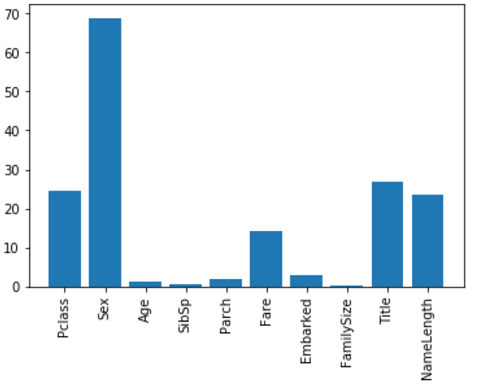
上图就是特征重要性的一个柱状图,发现Age等一些特征好像影响不大,和刚开始的假设有较大出入,那么这些没用的特征就可以删除掉,只保留有用的特征即可。
五、集成算法
使用集成算法来提升准确率
from sklearn.ensemble import GradientBoostingClassifier import numpy as np # The algorithms we want to ensemble. # We're using the more linear predictors for the logistic regression, and everything with the gradient boosting classifier. algorithms = [ [GradientBoostingClassifier(random_state=1, n_estimators=25, max_depth=3), ["Pclass", "Sex", "Age", "Fare", "Embarked", "FamilySize", "Title",]], [LogisticRegression(random_state=1,solver='liblinear'), ["Pclass", "Sex", "Fare", "FamilySize", "Title", "Age", "Embarked"]] ] # Initialize the cross validation folds kf = KFold(n_splits=3,shuffle=False, random_state=1) predictions = [] for train, test in kf.split(titanic): train_target = titanic["Survived"].iloc[train] full_test_predictions = [] # Make predictions for each algorithm on each fold for alg, predictors in algorithms: # Fit the algorithm on the training data. alg.fit(titanic[predictors].iloc[train,:], train_target) # Select and predict on the test fold. # The .astype(float) is necessary to convert the dataframe to all floats and avoid an sklearn error. test_predictions = alg.predict_proba(titanic[predictors].iloc[test,:].astype(float))[:,1] full_test_predictions.append(test_predictions) # Use a simple ensembling scheme -- just average the predictions to get the final classification. test_predictions = (full_test_predictions[0] + full_test_predictions[1]) / 2 # 两个分类器的平均结果 # Any value over .5 is assumed to be a 1 prediction, and below .5 is a 0 prediction. test_predictions[test_predictions <= .5] = 0 test_predictions[test_predictions > .5] = 1 predictions.append(test_predictions) # Put all the predictions together into one array. # 将所有的预测放在一个数组中 predictions = np.concatenate(predictions, axis=0) # Compute accuracy by comparing to the training data. accuracy = sum(predictions == titanic["Survived"]) / len(predictions) print(accuracy)
得到的准确率为:
0.8215488215488216
接下来用测试数据集来进行预测(注意:在测试数据集里面没有”Survived”这一列,所以我们得不到测试结果的准确率,只能进行预测)
titles = titanic_test["Name"].apply(get_title) # We're adding the Dona title to the mapping, because it's in the test set, but not the training set title_mapping = { "Mr": 1, "Miss": 2, "Mrs": 3, "Master": 4, "Dr": 5, "Rev": 6, "Major": 7, "Col": 7, "Mlle": 8, "Mme": 8, "Don": 9, "Lady": 10, "Countess": 10, "Jonkheer": 10, "Sir": 9, "Capt": 7, "Ms": 2, "Dona": 10 } for k, v in title_mapping.items(): titles[titles == k] = v titanic_test["Title"] = titles # Check the counts of each unique title. print(pandas.value_counts(titanic_test["Title"])) # Now, we add the family size column. titanic_test["FamilySize"] = titanic_test["SibSp"] + titanic_test["Parch"]
得到测试数据集里面Name里面称呼的次数:
1 240 2 79 3 72 4 21 7 2 6 2 10 1 5 1 Name: Title, dtype: int64
最终对测试数据集里面的乘客能否获救进行预测
predictors = [ "Pclass", "Sex", "Age", "Fare", "Embarked", "FamilySize", "Title" ] algorithms = [ [ GradientBoostingClassifier(random_state=1, n_estimators=25, max_depth=3), predictors ], [ LogisticRegression(random_state=1, solver='liblinear'), ["Pclass", "Sex", "Fare", "FamilySize", "Title", "Age", "Embarked"] ] ] full_predictions = [] for alg, predictors in algorithms: # Fit the algorithm using the full training data. alg.fit(titanic[predictors], titanic["Survived"]) # Predict using the test dataset. We have to convert all the columns to floats to avoid an error. predictions = alg.predict_proba( titanic_test[predictors].astype(float))[:, 1] predictions[predictions <= .5] = 0 predictions[predictions > .5] = 1 full_predictions.append(predictions) # The gradient boosting classifier generates better predictions, so we weight it higher. # predictions = (full_predictions[0] * 3 + full_predictions[1]) / 4 predictions
得到的结果(1表示能够获救,0表示不能被获救):
array([0., 0., 0., 0., 1., 0., 1., 0., 1., 0., 0., 0., 1., 0., 1., 1., 0., 0., 1., 1., 0., 0., 1., 0., 1., 0., 1., 0., 0., 0., 0., 0., 0., 1., 0., 0., 1., 1., 0., 0., 0., 0., 0., 1., 1., 0., 0., 0., 1., 0., 0., 0., 1., 1., 0., 0., 0., 0., 0., 1., 0., 0., 0., 1., 1., 1., 1., 0., 0., 1., 1., 0., 1., 0., 1., 1., 0., 1., 0., 1., 0., 0., 0., 0., 0., 0., 1., 1., 1., 1., 1., 0., 1., 0., 0., 0., 1., 0., 1., 0., 1., 0., 0., 0., 1., 0., 0., 0., 0., 0., 0., 1., 1., 1., 1., 0., 0., 1., 0., 1., 1., 0., 1., 0., 0., 1., 0., 1., 0., 0., 0., 1., 0., 0., 0., 0., 0., 0., 1., 0., 0., 1., 0., 0., 0., 0., 0., 0., 0., 0., 1., 0., 0., 0., 0., 0., 1., 1., 0., 1., 1., 0., 1., 0., 0., 1., 0., 0., 1., 1., 0., 0., 0., 0., 0., 1., 1., 0., 1., 1., 0., 0., 1., 0., 1., 0., 1., 0., 0., 0., 0., 0., 0., 0., 0., 0., 1., 1., 0., 1., 1., 0., 1., 1., 0., 0., 1., 0., 1., 0., 0., 0., 0., 1., 0., 0., 1., 0., 1., 0., 1., 0., 1., 0., 1., 1., 0., 1., 0., 0., 0., 1., 0., 0., 0., 0., 0., 0., 1., 1., 1., 1., 0., 0., 0., 0., 1., 0., 1., 1., 1., 0., 1., 0., 0., 0., 0., 0., 1., 0., 0., 0., 1., 1., 0., 0., 0., 0., 1., 0., 0., 0., 1., 1., 0., 1., 0., 0., 0., 0., 1., 0., 1., 1., 1., 0., 0., 0., 0., 0., 0., 1., 0., 0., 0., 0., 1., 0., 0., 0., 0., 0., 0., 0., 1., 1., 0., 0., 0., 0., 0., 0., 0., 1., 1., 1., 0., 0., 0., 0., 0., 0., 0., 0., 1., 0., 1., 0., 0., 0., 1., 0., 0., 1., 0., 0., 0., 0., 0., 0., 0., 0., 0., 1., 0., 1., 0., 1., 0., 1., 1., 0., 0., 0., 1., 0., 1., 0., 0., 1., 0., 1., 1., 0., 1., 0., 0., 1., 1., 0., 0., 1., 0., 0., 1., 1., 1., 0., 0., 0., 0., 0., 1., 1., 0., 1., 0., 0., 0., 0., 1., 1., 0., 0., 0., 1., 0., 1., 0., 0., 1., 0., 1., 1., 0., 0., 0., 0., 1., 1., 1., 1., 1., 0., 1., 0., 0., 0.])
六、总结
首先考虑数据集里面的所有特征,尽可能提取出来对结果有影响的一些信息。然后缺失值的处理,字符数据的映射,机器学习算法的改变,模型参数的优化,最后使用集成算法提升准确率。还包括对数据集的特征重要性的衡量和筛选。
